使用 PyTorch 构建自定义模型#
本 Notebook 演示了如何使用 PyTorch 在 GluonTS 中实现时间序列模型,使用 PyTorch Lightning 进行训练,并将其与 GluonTS 生态系统的其余部分结合使用,以进行数据加载、特征处理和模型评估。
[1]:
from typing import List, Optional, Callable, Iterable
from itertools import islice
[2]:
import numpy as np
import pandas as pd
from matplotlib import pyplot as plt
import matplotlib.dates as mdates
在本示例中,我们将使用“electricity”数据集,加载方法如下。
[3]:
from gluonts.dataset.repository import get_dataset
[4]:
dataset = get_dataset("electricity")
这是数据集训练部分中的第一条时间序列的样子
[5]:
date_formater = mdates.DateFormatter("%Y")

fig = plt.figure(figsize=(12, 8))
for idx, entry in enumerate(islice(dataset.train, 9)):
    ax = plt.subplot(3, 3, idx + 1)
    t = pd.date_range(
        start=entry["start"].to_timestamp(),
        periods=len(entry["target"]),
        freq=entry["start"].freq,
    )
    plt.plot(t, entry["target"])
    plt.xticks(pd.date_range(start="2011-12-31", periods=3, freq="AS"))
    ax.xaxis.set_major_formatter(date_formater)

使用 PyTorch 的概率前馈网络#
我们将使用一个相当简单的模型,它基于一个前馈网络,其输出层产生参数分布的参数。默认情况下,模型将使用 Student's t-分布,但这可以通过 distr_output 构造函数参数轻松自定义。
[6]:
import torch
import torch.nn as nn
[7]:
from gluonts.torch.model.predictor import PyTorchPredictor
from gluonts.torch.distributions import StudentTOutput
from gluonts.model.forecast_generator import DistributionForecastGenerator
[8]:
def mean_abs_scaling(context, min_scale=1e-5):
    return context.abs().mean(1).clamp(min_scale, None).unsqueeze(1)
[9]:
class FeedForwardNetwork(nn.Module):
    def __init__(
        self,
        prediction_length: int,
        context_length: int,
        hidden_dimensions: List[int],
        distr_output=StudentTOutput(),
        batch_norm: bool = False,
        scaling: Callable = mean_abs_scaling,
    ) -> None:
        super().__init__()

        assert prediction_length > 0
        assert context_length > 0
        assert len(hidden_dimensions) > 0

        self.prediction_length = prediction_length
        self.context_length = context_length
        self.hidden_dimensions = hidden_dimensions
        self.distr_output = distr_output
        self.batch_norm = batch_norm
        self.scaling = scaling

        dimensions = [context_length] + hidden_dimensions[:-1]

        modules = []
        for in_size, out_size in zip(dimensions[:-1], dimensions[1:]):
            modules += [self.__make_lin(in_size, out_size), nn.ReLU()]
            if batch_norm:
                modules.append(nn.BatchNorm1d(out_size))
        modules.append(
            self.__make_lin(dimensions[-1], prediction_length * hidden_dimensions[-1])
        )

        self.nn = nn.Sequential(*modules)
        self.args_proj = self.distr_output.get_args_proj(hidden_dimensions[-1])

    @staticmethod
    def __make_lin(dim_in, dim_out):
        lin = nn.Linear(dim_in, dim_out)
        torch.nn.init.uniform_(lin.weight, -0.07, 0.07)
        torch.nn.init.zeros_(lin.bias)
        return lin

    def forward(self, past_target):
        scale = self.scaling(past_target)
        scaled_past_target = past_target / scale
        nn_out = self.nn(scaled_past_target)
        nn_out_reshaped = nn_out.reshape(
            -1, self.prediction_length, self.hidden_dimensions[-1]
        )
        distr_args = self.args_proj(nn_out_reshaped)
        return distr_args, torch.zeros_like(scale), scale

    def get_predictor(self, input_transform, batch_size=32):
        return PyTorchPredictor(
            prediction_length=self.prediction_length,
            input_names=["past_target"],
            prediction_net=self,
            batch_size=batch_size,
            input_transform=input_transform,
            forecast_generator=DistributionForecastGenerator(self.distr_output),
        )
要使用 PyTorch Lightning 训练模型,我们只需扩展类并添加指定训练步骤如何工作的方法。有关如何完全自定义训练过程所需实现的接口的更多信息,请参阅 PyTorch Lightning 文档。
[10]:
import lightning.pytorch as pl
[11]:
class LightningFeedForwardNetwork(FeedForwardNetwork, pl.LightningModule):
    def __init__(self, *args, **kwargs):
        super().__init__(*args, **kwargs)

    def training_step(self, batch, batch_idx):
        past_target = batch["past_target"]
        future_target = batch["future_target"]

        assert past_target.shape[-1] == self.context_length
        assert future_target.shape[-1] == self.prediction_length

        distr_args, loc, scale = self(past_target)
        distr = self.distr_output.distribution(distr_args, loc, scale)
        loss = -distr.log_prob(future_target)

        return loss.mean()

    def configure_optimizers(self):
        optimizer = torch.optim.Adam(self.parameters(), lr=1e-3)
        return optimizer
现在我们可以实例化训练网络,并探索其参数集。
[12]:
context_length = 2 * 7 * 24
prediction_length = dataset.metadata.prediction_length
hidden_dimensions = [96, 48]
[13]:
net = LightningFeedForwardNetwork(
    prediction_length=prediction_length,
    context_length=context_length,
    hidden_dimensions=hidden_dimensions,
    distr_output=StudentTOutput(),
)
[14]:
sum(np.prod(p.shape) for p in net.parameters())
[14]:
144243
[15]:
for p in net.parameters():
    print(p.shape)
torch.Size([96, 336])
torch.Size([96])
torch.Size([1152, 96])
torch.Size([1152])
torch.Size([1, 48])
torch.Size([1])
torch.Size([1, 48])
torch.Size([1])
torch.Size([1, 48])
torch.Size([1])
定义训练数据加载器#
现在我们设置数据加载器,它将提供用于训练的数据批次。从原始数据集开始,数据加载器被配置为应用以下转换,这主要做两件事: * 将目标字段中的 nan 替换为虚拟值(零),并添加一个字段指示哪些值是实际观测到的,哪些是这样填充的。 * 从给定数据集中随机切出固定长度的训练实例;这些将由数据加载器本身堆叠成批次。
[16]:
from gluonts.dataset.field_names import FieldName
from gluonts.transform import (
    AddObservedValuesIndicator,
    InstanceSplitter,
    ExpectedNumInstanceSampler,
    TestSplitSampler,
)
[17]:
mask_unobserved = AddObservedValuesIndicator(
    target_field=FieldName.TARGET,
    output_field=FieldName.OBSERVED_VALUES,
)
[18]:
training_splitter = InstanceSplitter(
    target_field=FieldName.TARGET,
    is_pad_field=FieldName.IS_PAD,
    start_field=FieldName.START,
    forecast_start_field=FieldName.FORECAST_START,
    instance_sampler=ExpectedNumInstanceSampler(
        num_instances=1,
        min_future=prediction_length,
    ),
    past_length=context_length,
    future_length=prediction_length,
    time_series_fields=[FieldName.OBSERVED_VALUES],
)
[19]:
from gluonts.dataset.loader import TrainDataLoader
from gluonts.itertools import Cached
from gluonts.torch.batchify import batchify
[20]:
batch_size = 32
num_batches_per_epoch = 50
[21]:
data_loader = TrainDataLoader(
    # We cache the dataset, to make training faster
    Cached(dataset.train),
    batch_size=batch_size,
    stack_fn=batchify,
    transform=mask_unobserved + training_splitter,
    num_batches_per_epoch=num_batches_per_epoch,
)
训练模型#
现在我们可以使用 PyTorch Lightning 提供的工具来训练模型
[22]:
trainer = pl.Trainer(max_epochs=10)
trainer.fit(net, data_loader)
INFO: GPU available: False, used: False
INFO:lightning.pytorch.utilities.rank_zero:GPU available: False, used: False
INFO: TPU available: False, using: 0 TPU cores
INFO:lightning.pytorch.utilities.rank_zero:TPU available: False, using: 0 TPU cores
INFO: IPU available: False, using: 0 IPUs
INFO:lightning.pytorch.utilities.rank_zero:IPU available: False, using: 0 IPUs
INFO: HPU available: False, using: 0 HPUs
INFO:lightning.pytorch.utilities.rank_zero:HPU available: False, using: 0 HPUs
/opt/hostedtoolcache/Python/3.8.18/x64/lib/python3.8/site-packages/lightning/pytorch/trainer/connectors/logger_connector/logger_connector.py:67: Starting from v1.9.0, `tensorboardX` has been removed as a dependency of the `lightning.pytorch` package, due to potential conflicts with other packages in the ML ecosystem. For this reason, `logger=True` will use `CSVLogger` as the default logger, unless the `tensorboard` or `tensorboardX` packages are found. Please `pip install lightning[extra]` or one of them to enable TensorBoard support by default
WARNING: Missing logger folder: /home/runner/work/gluonts/gluonts/lightning_logs
WARNING:lightning.fabric.loggers.csv_logs:Missing logger folder: /home/runner/work/gluonts/gluonts/lightning_logs
INFO:
  | Name      | Type       | Params
-----------------------------------------
0 | nn        | Sequential | 144 K
1 | args_proj | PtArgProj  | 147
-----------------------------------------
144 K     Trainable params
0         Non-trainable params
144 K     Total params
0.577     Total estimated model params size (MB)
INFO:lightning.pytorch.callbacks.model_summary:
  | Name      | Type       | Params
-----------------------------------------
0 | nn        | Sequential | 144 K
1 | args_proj | PtArgProj  | 147
-----------------------------------------
144 K     Trainable params
0         Non-trainable params
144 K     Total params
0.577     Total estimated model params size (MB)
Epoch 9: | | 50/? [00:00<00:00, 87.44it/s, v_num=0]
INFO: `Trainer.fit` stopped: `max_epochs=10` reached.
INFO:lightning.pytorch.utilities.rank_zero:`Trainer.fit` stopped: `max_epochs=10` reached.
Epoch 9: | | 50/? [00:00<00:00, 86.03it/s, v_num=0]
从训练好的模型创建预测器并进行测试#
现在我们可以从模型中获取预测器,并用它来生成预测。
[23]:
prediction_splitter = InstanceSplitter(
    target_field=FieldName.TARGET,
    is_pad_field=FieldName.IS_PAD,
    start_field=FieldName.START,
    forecast_start_field=FieldName.FORECAST_START,
    instance_sampler=TestSplitSampler(),
    past_length=context_length,
    future_length=prediction_length,
    time_series_fields=[FieldName.OBSERVED_VALUES],
)
[24]:
predictor_pytorch = net.get_predictor(mask_unobserved + prediction_splitter)
例如,我们可以对测试数据集进行回测:接下来,make_evaluation_predictions 将从测试时间序列中切出末尾 prediction_length 个观测值,并使用给定的预测器获取相同时间范围的预测。
[25]:
from gluonts.evaluation import make_evaluation_predictions, Evaluator
[26]:
forecast_it, ts_it = make_evaluation_predictions(
    dataset=dataset.test, predictor=predictor_pytorch
)

forecasts_pytorch = list(f.to_sample_forecast() for f in forecast_it)
tss_pytorch = list(ts_it)
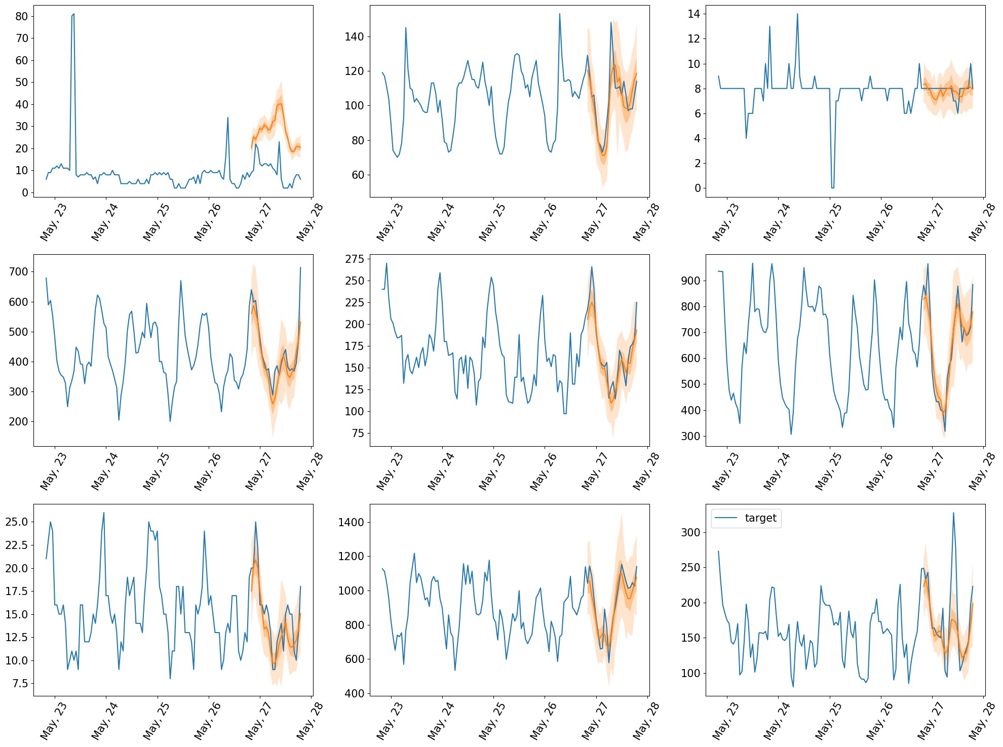
获得预测后,我们可以绘制它们
[27]:
plt.figure(figsize=(20, 15))
date_formater = mdates.DateFormatter("%b, %d")
plt.rcParams.update({"font.size": 15})

for idx, (forecast, ts) in islice(enumerate(zip(forecasts_pytorch, tss_pytorch)), 9):
    ax = plt.subplot(3, 3, idx + 1)
    plt.plot(ts[-5 * prediction_length :].to_timestamp(), label="target")
    forecast.plot()
    plt.xticks(rotation=60)
    ax.xaxis.set_major_formatter(date_formater)

plt.gcf().tight_layout()
plt.legend()
plt.show()
然后我们可以计算评估指标,总结模型在测试数据上的表现。
[28]:
evaluator = Evaluator(quantiles=[0.1, 0.5, 0.9])
[29]:
metrics_pytorch, _ = evaluator(tss_pytorch, forecasts_pytorch)
pd.DataFrame.from_records(metrics_pytorch, index=["FeedForward"]).transpose()
Running evaluation: 2247it [00:00, 26415.65it/s]
/opt/hostedtoolcache/Python/3.8.18/x64/lib/python3.8/site-packages/pandas/core/dtypes/astype.py:138: UserWarning: Warning: converting a masked element to nan.
  return arr.astype(dtype, copy=True)
[29]:
| FeedForward | |
|---|---|
| Coverage[0.1] | 7.617564e-02 |
| Coverage[0.5] | 4.742620e-01 |
| Coverage[0.9] | 9.205422e-01 |
| MAE_Coverage | 4.205422e-01 |
| MAPE | 1.483712e-01 |
| MASE | 9.660953e-01 |
| MSE | 3.635613e+06 |
| MSIS | 8.825237e+00 |
| ND | 9.193235e-02 |
| NRMSE | 7.993756e-01 |
| OWA | NaN |
| QuantileLoss[0.1] | 6.258573e+06 |
| QuantileLoss[0.5] | 1.182553e+07 |
| QuantileLoss[0.9] | 5.593065e+06 |
| RMSE | 1.906728e+03 |
| abs_error | 1.182553e+07 |
| abs_target_mean | 2.385272e+03 |
| abs_target_sum | 1.286330e+08 |
| mean_absolute_QuantileLoss | 7.892389e+06 |
| mean_wQuantileLoss | 6.135589e-02 |
| num_masked_target_values | 0.000000e+00 |
| sMAPE | 1.354325e-01 |
| seasonal_error | 1.894934e+02 |
| wQuantileLoss[0.1] | 4.865451e-02 |
| wQuantileLoss[0.5] | 9.193235e-02 |
| wQuantileLoss[0.9] | 4.348081e-02 |