下载此 Notebook

将数据集分割为训练集和测试集

在本 Notebook 中，我们将展示如何沿着时间分割数据集条目，以构建训练和测试数据子集（或训练/验证/测试）。具体来说，我们将使用 split 函数

from gluonts.dataset.split import split

这需要提供

• 要分割的 dataset；

• 一个 offset 或一个 date，但不能同时提供两者。提供这两个参数是为了让函数知道如何根据固定的整数偏移量或 pandas.Period 来切分训练数据和测试数据。

结果是，split 方法返回分割后的数据集，包括训练数据 training_dataset 以及一个知道如何生成输入/输出测试对的“测试模板”。

加载数据集

%matplotlib inline
import pandas as pd
import matplotlib.pyplot as plt

plt.rcParams["axes.grid"] = True
plt.rcParams["figure.figsize"] = (20, 3)

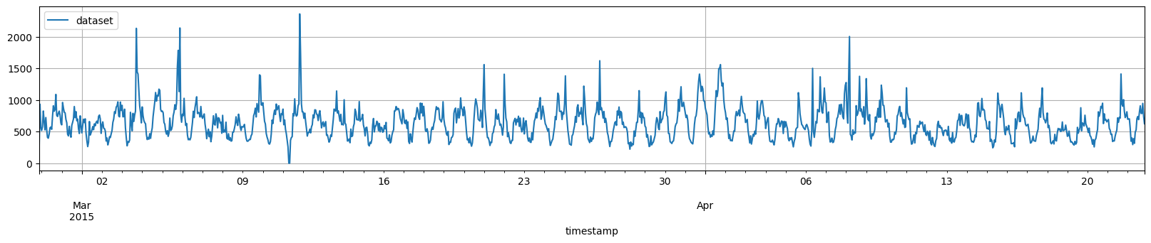
对于我们的示例，我们将使用以下 csv 文件中的数据，该文件原始采样频率为每 5 分钟，但我们将其重采样为每小时频率。请注意，这将创建一个包含单个时间序列的数据集，但我们在此展示的一切均适用于任何数据集，无论其包含多少时间序列。

url = "https://raw.githubusercontent.com/numenta/NAB/master/data/realTweets/Twitter_volume_AMZN.csv"
df = (
    pd.read_csv(url, header=0, index_col="timestamp", parse_dates=True)
    .resample("1H")
    .sum()
)

数据看起来像这样

df.plot()
plt.legend(["dataset"], loc="upper left")
plt.show()

使用 PandasDataset 将数据框转换为 GluonTS 数据集

from gluonts.dataset.pandas import PandasDataset

dataset = PandasDataset(df, target="value")

训练/测试分割

让我们定义一些辅助函数来可视化数据分割。

from gluonts.dataset.util import to_pandas


def highlight_entry(entry, color):
    start = entry["start"]
    end = entry["start"] + len(entry["target"])
    plt.axvspan(start, end, facecolor=color, alpha=0.2)


def plot_dataset_splitting(original_dataset, training_dataset, test_pairs):
    for original_entry, train_entry in zip(original_dataset, training_dataset):
        to_pandas(original_entry).plot()
        highlight_entry(train_entry, "red")
        plt.legend(["sub dataset", "training dataset"], loc="upper left")
        plt.show()

    for original_entry in original_dataset:
        for test_input, test_label in test_pairs:
            to_pandas(original_entry).plot()
            highlight_entry(test_input, "green")
            highlight_entry(test_label, "blue")
            plt.legend(["sub dataset", "test input", "test label"], loc="upper left")
            plt.show()

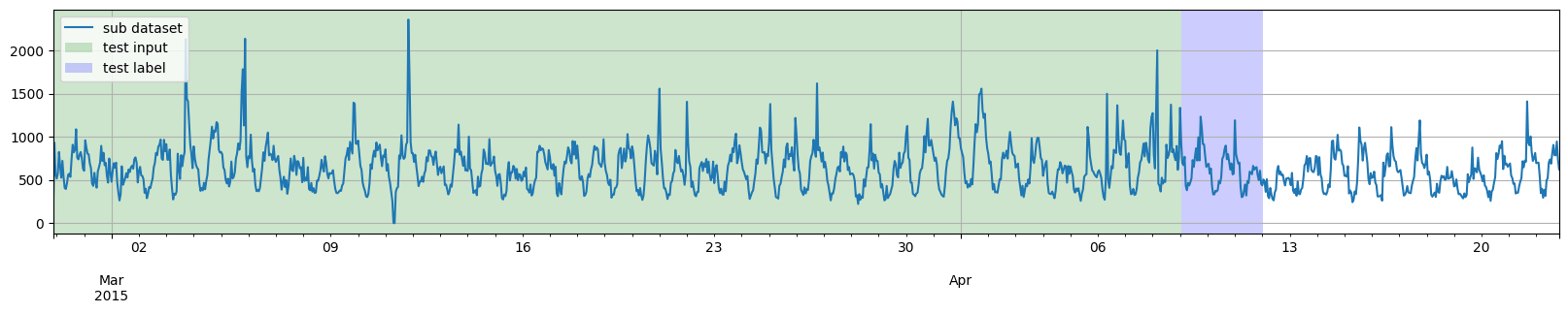
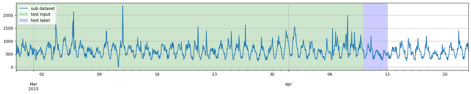
第一个例子，我们将选取到特定日期为止的训练数据，然后从该日期开始直接生成多个测试实例。

prediction_length = 3 * 24
training_dataset, test_template = split(
    dataset, date=pd.Period("2015-04-07 00:00:00", freq="1H")
)
test_pairs = test_template.generate_instances(
    prediction_length=prediction_length,
    windows=3,
)

plot_dataset_splitting(dataset, training_dataset, test_pairs)

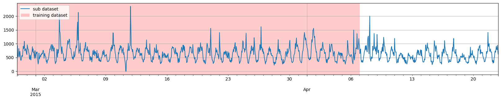
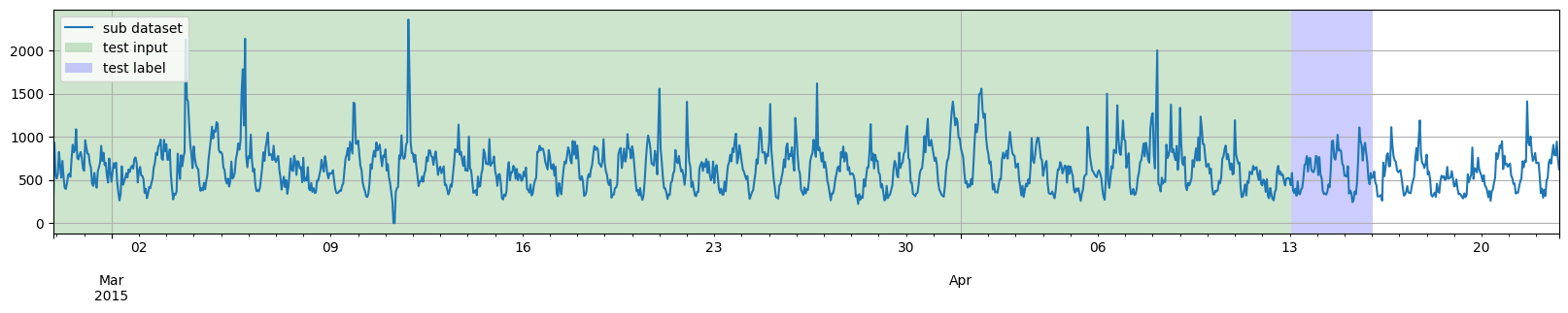
然而，我们并不一定需要将训练数据结束的日期与测试部分开始的日期对齐。因此，第二个例子，我们将选取到日期 2015-03-27 00:00:00 为止的训练数据，然后通过两次应用 split 函数，从日期 2015-04-07 00:00:00 开始生成多个测试实例。

training_dataset, _ = split(dataset, date=pd.Period("2015-03-28 00:00:00", freq="1H"))
_, test_template = split(dataset, date=pd.Period("2015-04-07 00:00:00", freq="1H"))
test_pairs = test_template.generate_instances(
    prediction_length=prediction_length,
    windows=3,
)

plot_dataset_splitting(dataset, training_dataset, test_pairs)

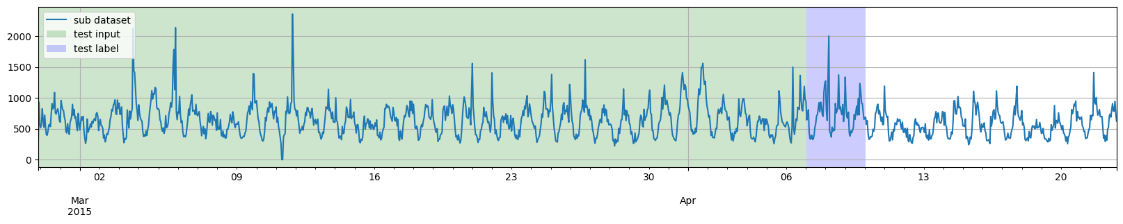
此外，我们也不一定需要将所有测试实例的时间完全对齐。因此，第三个例子，我们将在 generate_instances 函数中添加 distance 参数，以使测试实例相互重叠。

training_dataset, test_template = split(
    dataset, date=pd.Period("2015-04-07 00:00:00", freq="1H")
)
test_pairs = test_template.generate_instances(
    prediction_length=prediction_length,
    windows=3,
    distance=24,
)

plot_dataset_splitting(dataset, training_dataset, test_pairs)