扩展预测教程#
[1]:
%matplotlib inline
import mxnet as mx
from mxnet import gluon
import numpy as np
import pandas as pd
import matplotlib.pyplot as plt
import json
import os
from itertools import islice
from pathlib import Path
[2]:
mx.random.seed(0)
np.random.seed(0)
数据集#
使用 GluonTS 的首要要求是拥有合适的数据集。GluonTS 为希望尝试各种模块的实践者提供了三种不同的选项:
使用 GluonTS 提供的可用数据集
使用 GluonTS 创建人工数据集
将您自己的数据集转换为 GluonTS 友好格式
一般来说,数据集应满足一些最低格式要求才能与 GluonTS 兼容。特别是,它应该是一个可迭代的数据条目(时间序列)集合,并且每个条目应至少包含一个 target 字段,其中包含时间序列的实际值,以及一个 start 字段,表示时间序列的起始日期。本教程中我们将介绍更多可选字段。
GluonTS 提供的数据集格式合适,无需任何后处理即可使用。然而,自定义数据集需要转换。幸运的是,这项任务很容易。
GluonTS 中的可用数据集#
GluonTS 包含许多可用数据集。
[3]:
from gluonts.dataset.repository import get_dataset, dataset_names
from gluonts.dataset.util import to_pandas
[4]:
print(f"Available datasets: {dataset_names}")
Available datasets: ['constant', 'exchange_rate', 'solar-energy', 'electricity', 'traffic', 'exchange_rate_nips', 'electricity_nips', 'traffic_nips', 'solar_nips', 'wiki2000_nips', 'wiki-rolling_nips', 'taxi_30min', 'kaggle_web_traffic_with_missing', 'kaggle_web_traffic_without_missing', 'kaggle_web_traffic_weekly', 'm1_yearly', 'm1_quarterly', 'm1_monthly', 'nn5_daily_with_missing', 'nn5_daily_without_missing', 'nn5_weekly', 'tourism_monthly', 'tourism_quarterly', 'tourism_yearly', 'cif_2016', 'london_smart_meters_without_missing', 'wind_farms_without_missing', 'car_parts_without_missing', 'dominick', 'fred_md', 'pedestrian_counts', 'hospital', 'covid_deaths', 'kdd_cup_2018_without_missing', 'weather', 'm3_monthly', 'm3_quarterly', 'm3_yearly', 'm3_other', 'm4_hourly', 'm4_daily', 'm4_weekly', 'm4_monthly', 'm4_quarterly', 'm4_yearly', 'm5', 'uber_tlc_daily', 'uber_tlc_hourly', 'airpassengers', 'australian_electricity_demand', 'electricity_hourly', 'electricity_weekly', 'rideshare_without_missing', 'saugeenday', 'solar_10_minutes', 'solar_weekly', 'sunspot_without_missing', 'temperature_rain_without_missing', 'vehicle_trips_without_missing', 'ercot', 'ett_small_15min', 'ett_small_1h']
要下载内置数据集之一,只需调用 get_dataset 并提供上述名称之一。GluonTS 可以重用已保存的数据集,以便下次无需再次下载。
[5]:
dataset = get_dataset("m4_hourly")
数据集包含什么?#
一般来说,GluonTS 提供的数据集是包含三个主要成员的对象:
dataset.train是用于训练的数据条目的可迭代集合。每个条目对应一个时间序列。dataset.test是用于推理的数据条目的可迭代集合。测试数据集是训练数据集的扩展版本,其中包含每个时间序列末尾在训练期间未见过的窗口。该窗口的长度等于推荐的预测长度。dataset.metadata包含数据集的元数据,例如时间序列的频率、推荐的预测范围、关联的特征等。
首先,让我们看看训练数据集的第一个条目包含什么。我们应该预期每个条目至少有一个 target 字段和一个 start 字段,并且测试条目的 target 应有一个等于 prediction_length 的附加窗口。
[6]:
# get the first time series in the training set
train_entry = next(iter(dataset.train))
train_entry.keys()
[6]:
dict_keys(['target', 'start', 'feat_static_cat', 'item_id'])
我们观察到,除了必需字段外,还有一个 feat_static_cat 字段(我们可以安全地忽略 source 字段)。这表明数据集除了时间序列值外,还包含一些特征。现在,我们也将忽略此字段。稍后我们将详细解释它以及所有其他可选字段。
我们可以类似地检查测试数据集的第一个条目。我们应该预期字段与训练数据集完全相同。
[7]:
# get the first time series in the test set
test_entry = next(iter(dataset.test))
test_entry.keys()
[7]:
dict_keys(['target', 'start', 'feat_static_cat', 'item_id'])
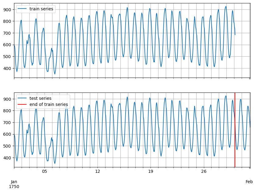
此外,我们应该预期 target 末尾会有一个长度等于 prediction_length 的附加窗口。为了更好地理解这意味着什么,我们可以可视化训练和测试时间序列。
[8]:
test_series = to_pandas(test_entry)
train_series = to_pandas(train_entry)

fig, ax = plt.subplots(2, 1, sharex=True, sharey=True, figsize=(10, 7))

train_series.plot(ax=ax[0])
ax[0].grid(which="both")
ax[0].legend(["train series"], loc="upper left")

test_series.plot(ax=ax[1])
ax[1].axvline(train_series.index[-1], color="r")  # end of train dataset
ax[1].grid(which="both")
ax[1].legend(["test series", "end of train series"], loc="upper left")

plt.show()
[9]:
print(
    f"Length of forecasting window in test dataset: {len(test_series) - len(train_series)}"
)
print(f"Recommended prediction horizon: {dataset.metadata.prediction_length}")
print(f"Frequency of the time series: {dataset.metadata.freq}")
Length of forecasting window in test dataset: 48
Recommended prediction horizon: 48
Frequency of the time series: H
创建人工数据集#
我们可以使用 ComplexSeasonalTimeSeries 模块轻松创建复杂的人工时间序列数据集。
[10]:
from gluonts.dataset.artificial import ComplexSeasonalTimeSeries
from gluonts.dataset.common import ListDataset
[11]:
artificial_dataset = ComplexSeasonalTimeSeries(
    num_series=10,
    prediction_length=21,
    freq_str="H",
    length_low=30,
    length_high=200,
    min_val=-10000,
    max_val=10000,
    is_integer=False,
    proportion_missing_values=0,
    is_noise=True,
    is_scale=True,
    percentage_unique_timestamps=1,
    is_out_of_bounds_date=True,
)
我们可以按如下方式访问人工数据集的一些重要元数据
[12]:
print(f"prediction length: {artificial_dataset.metadata.prediction_length}")
print(f"frequency: {artificial_dataset.metadata.freq}")
prediction length: 21
frequency: H
我们创建的人工数据集是一个字典列表。每个字典对应一个时间序列,并且应包含必需字段。
[13]:
print(f"type of train dataset: {type(artificial_dataset.train)}")
print(f"train dataset fields: {artificial_dataset.train[0].keys()}")
print(f"type of test dataset: {type(artificial_dataset.test)}")
print(f"test dataset fields: {artificial_dataset.test[0].keys()}")
type of train dataset: <class 'list'>
train dataset fields: dict_keys(['start', 'target', 'item_id'])
type of test dataset: <class 'list'>
test dataset fields: dict_keys(['start', 'target', 'item_id'])
为了使用人工创建的数据集(字典列表),我们需要将它们转换为 ListDataset 对象。
[14]:
train_ds = ListDataset(artificial_dataset.train, freq=artificial_dataset.metadata.freq)
[15]:
test_ds = ListDataset(artificial_dataset.test, freq=artificial_dataset.metadata.freq)
[16]:
train_entry = next(iter(train_ds))
train_entry.keys()
[16]:
dict_keys(['start', 'target', 'item_id'])
[17]:
test_entry = next(iter(test_ds))
test_entry.keys()
[17]:
dict_keys(['start', 'target', 'item_id'])
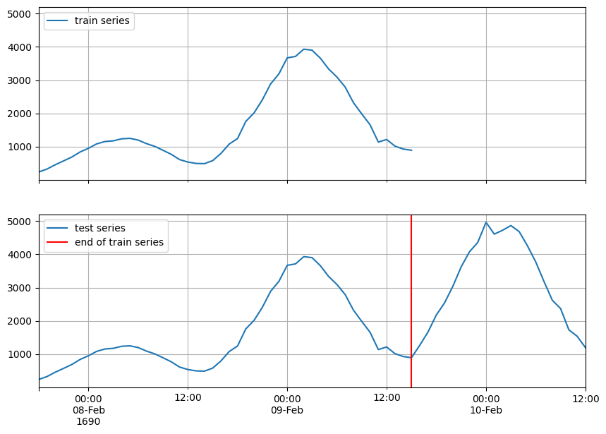
[18]:
test_series = to_pandas(test_entry)
train_series = to_pandas(train_entry)

fig, ax = plt.subplots(2, 1, sharex=True, sharey=True, figsize=(10, 7))

train_series.plot(ax=ax[0])
ax[0].grid(which="both")
ax[0].legend(["train series"], loc="upper left")

test_series.plot(ax=ax[1])
ax[1].axvline(train_series.index[-1], color="r")  # end of train dataset
ax[1].grid(which="both")
ax[1].legend(["test series", "end of train series"], loc="upper left")

plt.show()
使用您的时间序列和特征#
现在,我们将看到如何将任何带有任何关联特征的自定义数据集转换为 GluonTS 适用的格式。
如前所述,数据集要求至少包含 target 和 start 字段。但是,它可能包含更多字段。让我们看看所有可用字段是什么:
[19]:
from gluonts.dataset.field_names import FieldName
[20]:
[
    f"FieldName.{k} = '{v}'"
    for k, v in FieldName.__dict__.items()
    if not k.startswith("_")
]
[20]:
["FieldName.ITEM_ID = 'item_id'",
 "FieldName.INFO = 'info'",
 "FieldName.START = 'start'",
 "FieldName.TARGET = 'target'",
 "FieldName.FEAT_STATIC_CAT = 'feat_static_cat'",
 "FieldName.FEAT_STATIC_REAL = 'feat_static_real'",
 "FieldName.FEAT_DYNAMIC_CAT = 'feat_dynamic_cat'",
 "FieldName.FEAT_DYNAMIC_REAL = 'feat_dynamic_real'",
 "FieldName.PAST_FEAT_DYNAMIC_CAT = 'past_feat_dynamic_cat'",
 "FieldName.PAST_FEAT_DYNAMIC_REAL = 'past_feat_dynamic_real'",
 "FieldName.FEAT_DYNAMIC_REAL_LEGACY = 'dynamic_feat'",
 "FieldName.FEAT_DYNAMIC = 'feat_dynamic'",
 "FieldName.PAST_FEAT_DYNAMIC = 'past_feat_dynamic'",
 "FieldName.FEAT_TIME = 'time_feat'",
 "FieldName.FEAT_CONST = 'feat_dynamic_const'",
 "FieldName.FEAT_AGE = 'feat_dynamic_age'",
 "FieldName.OBSERVED_VALUES = 'observed_values'",
 "FieldName.IS_PAD = 'is_pad'",
 "FieldName.FORECAST_START = 'forecast_start'",
 "FieldName.TARGET_DIM_INDICATOR = 'target_dimension_indicator'"]
字段分为三类:必需字段、可选字段以及可由 Transformation 添加的字段(稍后解释)。
必需
start: 时间序列的开始日期target: 时间序列的值
可选
feat_static_cat: 静态(随时间不变)类别特征,维度等于特征数量的列表feat_static_real: 静态(随时间不变)实数值特征,维度等于特征数量的列表feat_dynamic_cat: 动态(随时间变化)类别特征,形状等于(特征数量,target 长度)的数组feat_dynamic_real: 动态(随时间变化)实数值特征,形状等于(特征数量,target 长度)的数组
由 Transformation 添加
time_feat: 时间相关特征,例如月份或日期feat_dynamic_const: 沿时间轴扩展常数值特征feat_dynamic_age: 年龄特征,即对于遥远过去的 timestamps 值较小,并且随着我们接近当前 timestamp 单调增加的特征observed_values: 观测值指示器,即如果值被观测到则等于 1,如果值缺失则等于 0 的特征is_pad: 每个时间步的指示器,显示是否已填充(如果长度不足)forecast_start: 预测开始日期
作为一个简单的例子,我们可以创建一个自定义数据集,看看如何使用其中的一些字段。该数据集包含 target、一个实数值动态特征(在此示例中,我们将其设置为前一个周期内的 target 值)以及一个静态类别特征,该特征指示我们用于创建 target 的正弦波类型(不同相位)。
[21]:
def create_dataset(num_series, num_steps, period=24, mu=1, sigma=0.3):
    # create target: noise + pattern
    # noise
    noise = np.random.normal(mu, sigma, size=(num_series, num_steps))

    # pattern - sinusoid with different phase
    sin_minusPi_Pi = np.sin(
        np.tile(np.linspace(-np.pi, np.pi, period), int(num_steps / period))
    )
    sin_Zero_2Pi = np.sin(
        np.tile(np.linspace(0, 2 * np.pi, 24), int(num_steps / period))
    )

    pattern = np.concatenate(
        (
            np.tile(sin_minusPi_Pi.reshape(1, -1), (int(np.ceil(num_series / 2)), 1)),
            np.tile(sin_Zero_2Pi.reshape(1, -1), (int(np.floor(num_series / 2)), 1)),
        ),
        axis=0,
    )

    target = noise + pattern

    # create time features: use target one period earlier, append with zeros
    feat_dynamic_real = np.concatenate(
        (np.zeros((num_series, period)), target[:, :-period]), axis=1
    )

    # create categorical static feats: use the sinusoid type as a categorical feature
    feat_static_cat = np.concatenate(
        (
            np.zeros(int(np.ceil(num_series / 2))),
            np.ones(int(np.floor(num_series / 2))),
        ),
        axis=0,
    )

    return target, feat_dynamic_real, feat_static_cat
[22]:
# define the parameters of the dataset
custom_ds_metadata = {
    "num_series": 100,
    "num_steps": 24 * 7,
    "prediction_length": 24,
    "freq": "1H",
    "start": [pd.Period("01-01-2019", freq="1H") for _ in range(100)],
}
[23]:
data_out = create_dataset(
    custom_ds_metadata["num_series"],
    custom_ds_metadata["num_steps"],
    custom_ds_metadata["prediction_length"],
)

target, feat_dynamic_real, feat_static_cat = data_out
我们可以通过简单地填充正确的字段来轻松创建训练和测试数据集。请记住,对于训练数据集,我们需要截断最后一个窗口。
[24]:
train_ds = ListDataset(
    [
        {
            FieldName.TARGET: target,
            FieldName.START: start,
            FieldName.FEAT_DYNAMIC_REAL: [fdr],
            FieldName.FEAT_STATIC_CAT: [fsc],
        }
        for (target, start, fdr, fsc) in zip(
            target[:, : -custom_ds_metadata["prediction_length"]],
            custom_ds_metadata["start"],
            feat_dynamic_real[:, : -custom_ds_metadata["prediction_length"]],
            feat_static_cat,
        )
    ],
    freq=custom_ds_metadata["freq"],
)
[25]:
test_ds = ListDataset(
    [
        {
            FieldName.TARGET: target,
            FieldName.START: start,
            FieldName.FEAT_DYNAMIC_REAL: [fdr],
            FieldName.FEAT_STATIC_CAT: [fsc],
        }
        for (target, start, fdr, fsc) in zip(
            target, custom_ds_metadata["start"], feat_dynamic_real, feat_static_cat
        )
    ],
    freq=custom_ds_metadata["freq"],
)
现在,我们可以检查训练和测试数据集的每个条目。我们应该预期它们包含以下字段:target、start、feat_dynamic_real 和 feat_static_cat。
[26]:
train_entry = next(iter(train_ds))
train_entry.keys()
[26]:
dict_keys(['target', 'start', 'feat_dynamic_real', 'feat_static_cat'])
[27]:
test_entry = next(iter(test_ds))
test_entry.keys()
[27]:
dict_keys(['target', 'start', 'feat_dynamic_real', 'feat_static_cat'])
[28]:
test_series = to_pandas(test_entry)
train_series = to_pandas(train_entry)

fig, ax = plt.subplots(2, 1, sharex=True, sharey=True, figsize=(10, 7))

train_series.plot(ax=ax[0])
ax[0].grid(which="both")
ax[0].legend(["train series"], loc="upper left")

test_series.plot(ax=ax[1])
ax[1].axvline(train_series.index[-1], color="r")  # end of train dataset
ax[1].grid(which="both")
ax[1].legend(["test series", "end of train series"], loc="upper left")

plt.show()
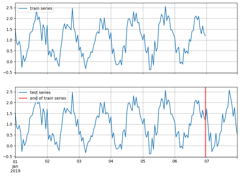
在本教程的其余部分,我们将使用自定义数据集
变换#
定义变换#
Transformation 的主要用例是特征处理,例如添加假日特征,以及定义数据集在训练和推理期间如何分割成合适的窗口。
一般来说,它接收数据集条目的可迭代集合,并将其转换为另一个可能包含更多字段的可迭代集合。变换通过对原始数据集定义一组“动作”来完成,具体取决于哪些对我们的模型有用。这些动作通常会创建一些附加特征或转换现有特征。例如,在下面我们添加了以下变换:
AddObservedValuesIndicator: 在数据集中创建observed_values字段,即添加一个特征,如果值被观测到则等于 1,如果值缺失则等于 0AddAgeFeature: 在数据集中创建feat_dynamic_age字段,即添加一个特征,对于遥远过去的 timestamps 值较小,并且随着我们接近当前 timestamp 单调增加
另一个可以使用的变换是 InstanceSplitter,它用于定义数据集如何在训练、验证或预测时分割成示例窗口。InstanceSplitter 配置如下(跳过显而易见的字段):
is_pad_field: 指示时间序列是否已填充(如果长度不足)train_sampler: 定义训练窗口如何被切割/采样time_series_fields: 包含需要与 target 以相同方式分割的时间依赖特征
[29]:
from gluonts.transform import (
    AddAgeFeature,
    AddObservedValuesIndicator,
    Chain,
    ExpectedNumInstanceSampler,
    InstanceSplitter,
    SetFieldIfNotPresent,
)
[30]:
def create_transformation(freq, context_length, prediction_length):
    return Chain(
        [
            AddObservedValuesIndicator(
                target_field=FieldName.TARGET,
                output_field=FieldName.OBSERVED_VALUES,
            ),
            AddAgeFeature(
                target_field=FieldName.TARGET,
                output_field=FieldName.FEAT_AGE,
                pred_length=prediction_length,
                log_scale=True,
            ),
            InstanceSplitter(
                target_field=FieldName.TARGET,
                is_pad_field=FieldName.IS_PAD,
                start_field=FieldName.START,
                forecast_start_field=FieldName.FORECAST_START,
                instance_sampler=ExpectedNumInstanceSampler(
                    num_instances=1,
                    min_future=prediction_length,
                ),
                past_length=context_length,
                future_length=prediction_length,
                time_series_fields=[
                    FieldName.FEAT_AGE,
                    FieldName.FEAT_DYNAMIC_REAL,
                    FieldName.OBSERVED_VALUES,
                ],
            ),
        ]
    )
变换数据集#
现在,我们可以通过将上述变换应用于我们创建的自定义数据集来创建一个变换对象。
[31]:
transformation = create_transformation(
    custom_ds_metadata["freq"],
    2 * custom_ds_metadata["prediction_length"],  # can be any appropriate value
    custom_ds_metadata["prediction_length"],
)
[32]:
train_tf = transformation(iter(train_ds), is_train=True)
[33]:
type(train_tf)
[33]:
generator
正如预期的那样,输出是另一个可迭代对象。我们可以轻松检查变换后数据集的条目中包含什么。InstanceSplitter 迭代变换后的数据集,通过随机选择一个时间序列及其上的一个起始点来切割窗口(这种“随机性”由 instance_sampler 定义)。
[34]:
train_tf_entry = next(iter(train_tf))
[k for k in train_tf_entry.keys()]
[34]:
['start',
 'feat_static_cat',
 'past_feat_dynamic_age',
 'future_feat_dynamic_age',
 'past_feat_dynamic_real',
 'future_feat_dynamic_real',
 'past_observed_values',
 'future_observed_values',
 'past_target',
 'future_target',
 'past_is_pad',
 'forecast_start']
变换器已完成我们要求的操作。特别是,它添加了:
一个用于观测值的字段(
observed_values)一个用于年龄特征的字段(
feat_dynamic_age)一些额外的有用字段(
past_is_pad,forecast_start)
它还做了一件重要的事情:它将窗口分割为过去和未来,并为所有时间依赖字段添加了相应的 前缀。这样,我们可以轻松地使用例如 past_target 字段作为输入,并使用 future_target 字段计算预测误差。当然,过去的长度等于 context_length,未来的长度等于 prediction_length。
[35]:
print(f"past target shape: {train_tf_entry['past_target'].shape}")
print(f"future target shape: {train_tf_entry['future_target'].shape}")
print(f"past observed values shape: {train_tf_entry['past_observed_values'].shape}")
print(f"future observed values shape: {train_tf_entry['future_observed_values'].shape}")
print(f"past age feature shape: {train_tf_entry['past_feat_dynamic_age'].shape}")
print(f"future age feature shape: {train_tf_entry['future_feat_dynamic_age'].shape}")
print(train_tf_entry["feat_static_cat"])
past target shape: (48,)
future target shape: (24,)
past observed values shape: (48,)
future observed values shape: (24,)
past age feature shape: (48, 1)
future age feature shape: (24, 1)
[0]
仅作比较,让我们再次看看变换前原始数据集中的字段是什么
[36]:
[k for k in next(iter(train_ds)).keys()]
[36]:
['target', 'start', 'feat_dynamic_real', 'feat_static_cat']
现在,我们可以继续看看测试数据集是如何分割的。正如我们所见,变换将窗口分割为过去和未来。然而,在推理过程中(变换中的 is_train=False),splitter 总是截取数据集的最后一个窗口(长度为 context_length),以便用于预测后续长度为 prediction_length 的未知值。
那么,既然我们不知道未来的 target,测试数据集是如何分割为过去和未来的呢?时间依赖特征又如何呢?
[37]:
test_tf = transformation(iter(test_ds), is_train=False)
[38]:
test_tf_entry = next(iter(test_tf))
[k for k in test_tf_entry.keys()]
[38]:
['start',
 'feat_static_cat',
 'past_feat_dynamic_age',
 'future_feat_dynamic_age',
 'past_feat_dynamic_real',
 'future_feat_dynamic_real',
 'past_observed_values',
 'future_observed_values',
 'past_target',
 'future_target',
 'past_is_pad',
 'forecast_start']
[39]:
print(f"past target shape: {test_tf_entry['past_target'].shape}")
print(f"future target shape: {test_tf_entry['future_target'].shape}")
print(f"past observed values shape: {test_tf_entry['past_observed_values'].shape}")
print(f"future observed values shape: {test_tf_entry['future_observed_values'].shape}")
print(f"past age feature shape: {test_tf_entry['past_feat_dynamic_age'].shape}")
print(f"future age feature shape: {test_tf_entry['future_feat_dynamic_age'].shape}")
print(test_tf_entry["feat_static_cat"])
past target shape: (48,)
future target shape: (24,)
past observed values shape: (48,)
future observed values shape: (24,)
past age feature shape: (48, 1)
future age feature shape: (24, 1)
[0]
未来的 target 是空的,但特征不是空的——我们总是假设我们知道未来的特征!
我们在这里手动完成的所有事情都由一个内部块 DataLoader 完成。它将原始数据集(以适当的格式)和变换对象作为输入,并按批次输出变换后的可迭代数据集。我们唯一需要担心的是正确设置变换字段!
训练现有模型#
GluonTS 附带了许多预构建模型。用户只需配置一些超参数即可。现有模型侧重于(但不限于)概率预测。概率预测是以概率分布形式进行的预测,而不仅仅是单一的点估计。在估计出预测范围内每个时间步的未来分布后,我们可以从每个时间步的分布中抽取样本,从而创建一条“样本路径”,这可以被视为未来的一种可能实现。实际上,我们抽取多个样本并创建多条样本路径,可用于可视化、模型评估、推导统计量等。
配置估计器#
我们将从 GluonTS 的预构建前馈神经网络估计器开始,这是一个简单但功能强大的预测模型。我们将使用此模型演示训练模型、生成预测和评估结果的过程。
GluonTS 的内置前馈神经网络(SimpleFeedForwardEstimator)接受长度为 context_length 的输入窗口,并预测后续 prediction_length 个值的分布。在 GluonTS 的术语中,前馈神经网络模型是 Estimator 的一个示例。在 GluonTS 中,Estimator 对象表示预测模型及其系数、权重等详细信息。
一般来说,每个估计器(预构建或自定义)都由许多超参数配置,这些超参数可以是所有估计器共有的(但不强制),例如 prediction_length,也可以是特定于特定估计器的(例如,神经网络的层数或 CNN 中的步幅)。
最后,每个估计器由 Trainer 配置,它定义了模型的训练方式,即 epoch 数、学习率等。
[40]:
from gluonts.mx import SimpleFeedForwardEstimator, Trainer
[41]:
estimator = SimpleFeedForwardEstimator(
    num_hidden_dimensions=[10],
    prediction_length=custom_ds_metadata["prediction_length"],
    context_length=2 * custom_ds_metadata["prediction_length"],
    trainer=Trainer(
        ctx="cpu",
        epochs=5,
        learning_rate=1e-3,
        hybridize=False,
        num_batches_per_epoch=100,
    ),
)
获取预测器#
在指定了所有必要的超参数来配置我们的估计器后,我们可以使用训练数据集 dataset.train 调用估计器的 train 方法来训练它。训练算法返回一个拟合好的模型(在 GluonTS 的术语中称为 Predictor),该模型可用于构建预测。
这里需要强调的是,如上所述的单个模型是在训练数据集 train_ds 中包含的所有时间序列上进行训练的。这产生了一个全局模型,适用于预测 train_ds 中的所有时间序列以及可能未见过的相关时间序列。
[42]:
predictor = estimator.train(train_ds)
100%|██████████| 100/100 [00:00<00:00, 121.53it/s, epoch=1/5, avg_epoch_loss=1.28]
100%|██████████| 100/100 [00:00<00:00, 124.61it/s, epoch=2/5, avg_epoch_loss=0.735]
100%|██████████| 100/100 [00:00<00:00, 122.58it/s, epoch=3/5, avg_epoch_loss=0.677]
100%|██████████| 100/100 [00:00<00:00, 124.03it/s, epoch=4/5, avg_epoch_loss=0.644]
100%|██████████| 100/100 [00:00<00:00, 136.28it/s, epoch=5/5, avg_epoch_loss=0.605]
保存/加载现有模型#
拟合好的模型,即 Predictor,可以轻松保存和加载。
[43]:
# save the trained model in tmp/
from pathlib import Path

predictor.serialize(Path("/tmp/"))
WARNING:root:Serializing RepresentableBlockPredictor instances does not save the prediction network structure in a backwards-compatible manner. Be careful not to use this method in production.
[44]:
# loads it back
from gluonts.model.predictor import Predictor

predictor_deserialized = Predictor.deserialize(Path("/tmp/"))
评估#
获取预测结果#
有了预测器,我们现在可以预测 dataset.test 的最后一个窗口并评估我们模型的性能。
GluonTS 提供了 make_evaluation_predictions 函数,它自动化了预测和模型评估的过程。大致而言,该函数执行以下步骤:
移除我们要预测的
dataset.test中长度为prediction_length的最后一个窗口估计器使用剩余数据来预测(以样本路径的形式)刚刚移除的“未来”窗口
模块输出预测样本路径和
dataset.test(作为 python 生成器对象)
[45]:
from gluonts.evaluation import make_evaluation_predictions
[46]:
forecast_it, ts_it = make_evaluation_predictions(
    dataset=test_ds,  # test dataset
    predictor=predictor,  # predictor
    num_samples=100,  # number of sample paths we want for evaluation
)
首先,我们可以将这些生成器转换为列表,以便简化后续计算。
[47]:
forecasts = list(forecast_it)
tss = list(ts_it)
我们可以检查这些列表的第一个元素(对应于数据集的第一个时间序列)。让我们从包含时间序列的列表开始,即 tss。我们预期 tss 的第一个条目包含 test_ds 的第一个时间序列的(target)。
[48]:
# first entry of the time series list
ts_entry = tss[0]
[49]:
# first 5 values of the time series (convert from pandas to numpy)
np.array(ts_entry[:5]).reshape(
    -1,
)
[49]:
array([1.5292157 , 0.85025036, 0.7740374 , 0.941432  , 0.6723822 ],
      dtype=float32)
[50]:
# first entry of test_ds
test_ds_entry = next(iter(test_ds))
[51]:
# first 5 values
test_ds_entry["target"][:5]
[51]:
array([1.5292157 , 0.85025036, 0.7740374 , 0.941432  , 0.6723822 ],
      dtype=float32)
forecast 列表中的条目稍微复杂一些。它们是包含所有样本路径的对象,形式为 numpy.ndarray,维度为 (num_samples, prediction_length),还包含预测的开始日期、时间序列的频率等。只需调用预测对象的相应属性即可访问所有这些信息。
[52]:
# first entry of the forecast list
forecast_entry = forecasts[0]
[53]:
print(f"Number of sample paths: {forecast_entry.num_samples}")
print(f"Dimension of samples: {forecast_entry.samples.shape}")
print(f"Start date of the forecast window: {forecast_entry.start_date}")
print(f"Frequency of the time series: {forecast_entry.freq}")
Number of sample paths: 100
Dimension of samples: (100, 24)
Start date of the forecast window: 2019-01-07 00:00
Frequency of the time series: <Hour>
我们还可以进行计算来汇总样本路径,例如计算预测窗口中每个 24 个时间步的均值或分位数。
[54]:
print(f"Mean of the future window:\n {forecast_entry.mean}")
print(f"0.5-quantile (median) of the future window:\n {forecast_entry.quantile(0.5)}")
Mean of the future window:
 [ 0.90765196  0.5002642   0.58970827  0.39372978  0.09580009  0.05871432
 -0.09855336  0.21287599  0.06411848  0.36389527  0.6184984   0.82686234
  1.1362944   1.4422988   1.5806047   1.885066    1.6728904   1.8457131
  2.0097268   1.7956799   1.6775795   1.587245    1.2241242   1.0475011 ]
0.5-quantile (median) of the future window:
 [ 9.2138731e-01  5.3099197e-01  5.4954773e-01  3.5585621e-01
  1.3284978e-01  5.4421678e-02 -5.3116154e-02  1.7734313e-01
 -1.0389383e-03  3.8981181e-01  6.4071041e-01  8.7102258e-01
  1.1050647e+00  1.2608457e+00  1.5636476e+00  1.9202025e+00
  1.7487336e+00  1.8408449e+00  2.0478199e+00  1.7664530e+00
  1.7128807e+00  1.6053847e+00  1.2772603e+00  1.0452789e+00]
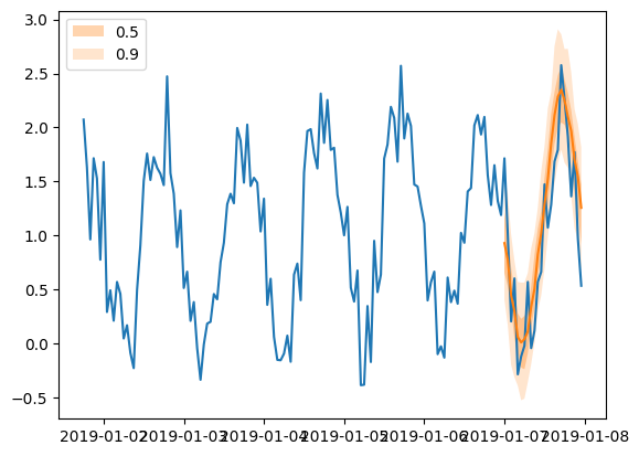
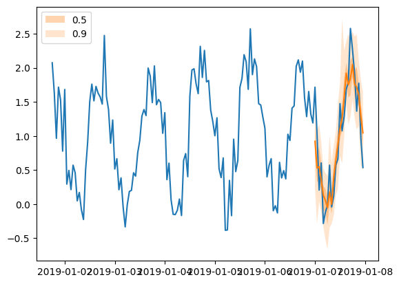
Forecast 对象有一个 plot 方法,可以将预测路径汇总为均值、预测区间等。预测区间以不同的颜色阴影显示,形成“扇形图”。
[55]:
plt.plot(ts_entry[-150:].to_timestamp())
forecast_entry.plot(show_label=True)
plt.legend()
[55]:
<matplotlib.legend.Legend at 0x7f24980497f0>
计算评估指标#
我们还可以数值地评估预测的质量。在 GluonTS 中,Evaluator 类可以计算总体性能指标,以及每个时间序列的指标(这对于分析异构时间序列的性能非常有用)。
[56]:
from gluonts.evaluation import Evaluator
[57]:
evaluator = Evaluator(quantiles=[0.1, 0.5, 0.9])
agg_metrics, item_metrics = evaluator(tss, forecasts)
Running evaluation: 100it [00:00, 2858.91it/s]
总体指标聚合了时间步和时间序列。
[58]:
print(json.dumps(agg_metrics, indent=4))
{
    "MSE": 0.11030595362186432,
    "abs_error": 631.219958782196,
    "abs_target_sum": 2505.765546798706,
    "abs_target_mean": 1.044068977832794,
    "seasonal_error": 0.3378558193842571,
    "MASE": 0.7856021114063411,
    "MAPE": 2.2423562081654866,
    "sMAPE": 0.5366955331961314,
    "MSIS": 5.561884554254895,
    "num_masked_target_values": 0.0,
    "QuantileLoss[0.1]": 274.70157045163216,
    "Coverage[0.1]": 0.09208333333333334,
    "QuantileLoss[0.5]": 631.2199574247934,
    "Coverage[0.5]": 0.4904166666666667,
    "QuantileLoss[0.9]": 295.76119372472164,
    "Coverage[0.9]": 0.8820833333333331,
    "RMSE": 0.332123401195797,
    "NRMSE": 0.3181048457978281,
    "ND": 0.2519070308028716,
    "wQuantileLoss[0.1]": 0.10962780249037385,
    "wQuantileLoss[0.5]": 0.25190703026115985,
    "wQuantileLoss[0.9]": 0.11803226926101591,
    "mean_absolute_QuantileLoss": 400.5609072003824,
    "mean_wQuantileLoss": 0.15985570067084987,
    "MAE_Coverage": 0.39402777777777764,
    "OWA": NaN
}
个体指标仅聚合时间步。
[59]:
item_metrics.head()
[59]:
| item_id | forecast_start | 均方误差 | 绝对误差 | 目标绝对值之和 | 目标绝对值均值 | 季节性误差 | MASE | MAPE | sMAPE | 被遮掩的目标值数量 | ND | MSIS | 分位数损失[0.1] | 覆盖率[0.1] | 分位数损失[0.5] | 覆盖率[0.5] | 分位数损失[0.9] | 覆盖率[0.9] | |
|---|---|---|---|---|---|---|---|---|---|---|---|---|---|---|---|---|---|---|---|
| 0 | 无 | 2019-01-07 00:00 | 0.123998 | 7.011340 | 24.638548 | 1.026606 | 0.351642 | 0.830787 | 0.627694 | 0.607183 | 0.0 | 0.284568 | 5.906248 | 2.286915 | 0.083333 | 7.011340 | 0.541667 | 3.406847 | 0.875000 |
| 1 | 无 | 2019-01-07 00:00 | 0.109331 | 5.898170 | 22.178631 | 0.924110 | 0.340241 | 0.722302 | 1.439482 | 0.555920 | 0.0 | 0.265939 | 5.646115 | 2.598318 | 0.083333 | 5.898170 | 0.666667 | 3.049512 | 0.916667 |
| 2 | 无 | 2019-01-07 00:00 | 0.150442 | 6.913772 | 26.601139 | 1.108381 | 0.323560 | 0.890326 | 0.419949 | 0.536978 | 0.0 | 0.259905 | 6.923015 | 3.400284 | 0.125000 | 6.913772 | 0.500000 | 3.971697 | 0.791667 |
| 3 | 无 | 2019-01-07 00:00 | 0.124376 | 6.302595 | 22.502333 | 0.937597 | 0.311026 | 0.844329 | 1.099858 | 0.609671 | 0.0 | 0.280086 | 7.677102 | 3.067686 | 0.208333 | 6.302595 | 0.583333 | 3.414130 | 0.958333 |
| 4 | 无 | 2019-01-07 00:00 | 0.073736 | 4.519842 | 25.864388 | 1.077683 | 0.313119 | 0.601453 | 0.920273 | 0.425719 | 0.0 | 0.174752 | 6.257542 | 2.332712 | 0.041667 | 4.519842 | 0.500000 | 2.810995 | 0.916667 |
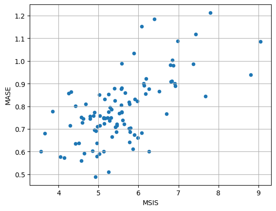
[60]:
item_metrics.plot(x="MSIS", y="MASE", kind="scatter")
plt.grid(which="both")
plt.show()
创建您自己的模型#
要创建我们自己的预测模型,我们需要:
定义训练和预测网络
定义一个新的估计器,指定任何数据处理并使用网络
训练和预测网络可以任意复杂,但应遵循一些基本规则:
两者都应有一个
hybrid_forward方法,定义网络被调用时应发生什么训练网络的
hybrid_forward应基于预测和真实值返回一个损失预测网络的
hybrid_forward应返回预测结果
估计器还应包含以下方法:
create_transformation, 定义所有数据预处理变换(如添加特征)create_training_data_loader, 构建用于训练的数据加载器,从给定数据集中提供批次数据create_training_network, 返回配置了所有必要超参数的训练网络create_predictor, 创建预测网络,并返回一个Predictor对象
如果需要接受验证数据集以计算某些验证指标,则还应定义以下内容:
create_validation_data_loader
一个 Predictor 定义了给定预测器的 predictor.predict 方法。此方法接收测试数据集,将其通过预测网络进行预测,并生成预测结果。您可以将 Predictor 对象视为预测网络的包装器,它定义了其 predict 方法。
在本节中,我们将从创建一个仅限于点预测的前馈网络开始,保持简单。然后,我们将通过将其扩展到概率预测、考虑时间序列的特征和缩放来增加网络的复杂性,最后将其替换为 RNN。
我们需要强调,以下模型的实现方式以及所有设计选择既不是强制性的,也未必是最佳的。它们唯一目的是提供构建模型的指导和提示。
使用简单前馈网络进行点预测#
我们可以创建一个简单的训练网络,该网络定义了一个神经网络,它接受长度为 context_length 的窗口作为输入,并预测维度为 prediction_length 的后续窗口(因此,网络的输出维度是 prediction_length)。训练网络的 hybrid_forward 方法返回 L1 损失的均值。
预测网络与训练网络相同(且应相同,通过继承类实现),其 hybrid_forward 方法返回预测结果。
[61]:
class MyNetwork(gluon.HybridBlock):
    def __init__(self, prediction_length, num_cells, **kwargs):
        super().__init__(**kwargs)
        self.prediction_length = prediction_length
        self.num_cells = num_cells

        with self.name_scope():
            # Set up a 3 layer neural network that directly predicts the target values
            self.nn = mx.gluon.nn.HybridSequential()
            self.nn.add(mx.gluon.nn.Dense(units=self.num_cells, activation="relu"))
            self.nn.add(mx.gluon.nn.Dense(units=self.num_cells, activation="relu"))
            self.nn.add(
                mx.gluon.nn.Dense(units=self.prediction_length, activation="softrelu")
            )


class MyTrainNetwork(MyNetwork):
    def hybrid_forward(self, F, past_target, future_target):
        prediction = self.nn(past_target)
        # calculate L1 loss with the future_target to learn the median
        return (prediction - future_target).abs().mean(axis=-1)


class MyPredNetwork(MyTrainNetwork):
    # The prediction network only receives past_target and returns predictions
    def hybrid_forward(self, F, past_target):
        prediction = self.nn(past_target)
        return prediction.expand_dims(axis=1)
估计器类由一些超参数配置并实现了所需的方法。
[62]:
from functools import partial
from mxnet.gluon import HybridBlock
from gluonts.core.component import validated
from gluonts.dataset.loader import TrainDataLoader
from gluonts.model.predictor import Predictor
from gluonts.mx import (
    batchify,
    copy_parameters,
    get_hybrid_forward_input_names,
    GluonEstimator,
    RepresentableBlockPredictor,
    Trainer,
)
from gluonts.transform import (
    ExpectedNumInstanceSampler,
    Transformation,
    InstanceSplitter,
    TestSplitSampler,
    SelectFields,
    Chain,
)
[63]:
class MyEstimator(GluonEstimator):
    @validated()
    def __init__(
        self,
        prediction_length: int,
        context_length: int,
        num_cells: int,
        batch_size: int = 32,
        trainer: Trainer = Trainer(),
    ) -> None:
        super().__init__(trainer=trainer, batch_size=batch_size)
        self.prediction_length = prediction_length
        self.context_length = context_length
        self.num_cells = num_cells

    def create_transformation(self):
        return Chain([])

    def create_training_data_loader(self, dataset, **kwargs):
        instance_splitter = InstanceSplitter(
            target_field=FieldName.TARGET,
            is_pad_field=FieldName.IS_PAD,
            start_field=FieldName.START,
            forecast_start_field=FieldName.FORECAST_START,
            instance_sampler=ExpectedNumInstanceSampler(
                num_instances=1, min_future=self.prediction_length
            ),
            past_length=self.context_length,
            future_length=self.prediction_length,
        )
        input_names = get_hybrid_forward_input_names(MyTrainNetwork)
        return TrainDataLoader(
            dataset=dataset,
            transform=instance_splitter + SelectFields(input_names),
            batch_size=self.batch_size,
            stack_fn=partial(batchify, ctx=self.trainer.ctx, dtype=self.dtype),
            **kwargs,
        )

    def create_training_network(self) -> MyTrainNetwork:
        return MyTrainNetwork(
            prediction_length=self.prediction_length, num_cells=self.num_cells
        )

    def create_predictor(
        self, transformation: Transformation, trained_network: HybridBlock
    ) -> Predictor:
        prediction_splitter = InstanceSplitter(
            target_field=FieldName.TARGET,
            is_pad_field=FieldName.IS_PAD,
            start_field=FieldName.START,
            forecast_start_field=FieldName.FORECAST_START,
            instance_sampler=TestSplitSampler(),
            past_length=self.context_length,
            future_length=self.prediction_length,
        )

        prediction_network = MyPredNetwork(
            prediction_length=self.prediction_length, num_cells=self.num_cells
        )

        copy_parameters(trained_network, prediction_network)

        return RepresentableBlockPredictor(
            input_transform=transformation + prediction_splitter,
            prediction_net=prediction_network,
            batch_size=self.batch_size,
            prediction_length=self.prediction_length,
            ctx=self.trainer.ctx,
        )
定义了训练和预测网络以及估计器类后,我们可以遵循与现有模型完全相同的步骤,即通过将所有必需的超参数传递给估计器类来指定我们的估计器,通过调用其 train 方法来训练估计器以创建预测器,最后使用 make_evaluation_predictions 函数生成我们的预测结果。
[64]:
estimator = MyEstimator(
    prediction_length=custom_ds_metadata["prediction_length"],
    context_length=2 * custom_ds_metadata["prediction_length"],
    num_cells=40,
    trainer=Trainer(
        ctx="cpu",
        epochs=5,
        learning_rate=1e-3,
        hybridize=False,
        num_batches_per_epoch=100,
    ),
)
估计器可以使用我们的训练数据集 train_ds 进行训练,只需调用其 train 方法即可。训练完成后将返回一个预测器,可用于预测。
[65]:
predictor = estimator.train(train_ds)
100%|██████████| 100/100 [00:00<00:00, 257.30it/s, epoch=1/5, avg_epoch_loss=0.48]
100%|██████████| 100/100 [00:00<00:00, 268.75it/s, epoch=2/5, avg_epoch_loss=0.319]
100%|██████████| 100/100 [00:00<00:00, 288.90it/s, epoch=3/5, avg_epoch_loss=0.302]
100%|██████████| 100/100 [00:00<00:00, 296.54it/s, epoch=4/5, avg_epoch_loss=0.289]
100%|██████████| 100/100 [00:00<00:00, 284.35it/s, epoch=5/5, avg_epoch_loss=0.288]
[66]:
forecast_it, ts_it = make_evaluation_predictions(
    dataset=test_ds,  # test dataset
    predictor=predictor,  # predictor
    num_samples=100,  # number of sample paths we want for evaluation
)
[67]:
forecasts = list(forecast_it)
tss = list(ts_it)
[68]:
plt.plot(tss[0][-150:].to_timestamp())
forecasts[0].plot(show_label=True)
plt.legend()
[68]:
<matplotlib.legend.Legend at 0x7f2498018880>
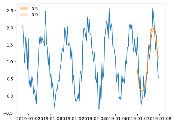
请注意,我们在预测结果中实际上看不到任何预测区间。这是预料之中的,因为我们定义的模型不进行概率预测,它只给出点估计。在这种网络中要求 100 条样本路径(在 make_evaluation_predictions 中定义)时,我们得到 100 次相同的输出。
概率预测#
模型如何学习分布?#
概率预测要求我们学习时间序列未来值的分布,而不是像点预测那样仅学习值本身。为此,我们需要指定未来值遵循的分布类型。GluonTS 提供了多种不同的分布,涵盖了许多用例,例如高斯分布、学生 t 分布和均匀分布等。
为了学习分布,我们需要学习其参数。例如,在我们假设高斯分布的简单情况下,我们需要学习完全指定该分布的均值和方差。
GluonTS 中可用的每种分布都由相应的 Distribution 类(例如 Gaussian)定义。此类定义了(除其他外)分布的参数、其(对数)似然以及采样方法(给定参数)。
然而,如何将模型与此类分布连接并学习其参数并不直接。为此,每种分布都附带一个 DistributionOutput 类(例如 GaussianOutput)。此类用于将模型与分布连接起来。其主要用途是将模型的输出映射到分布的参数。您可以将其视为模型顶部的附加投影层。此层的参数与网络的其余部分一起优化。
通过包含此投影层,我们的模型有效地学习了每个时间步的(选择的)分布参数。此类模型通常通过选择所选分布的负对数似然作为损失函数进行优化。优化模型并学习参数后,我们可以从学习到的分布中采样或推导出任何其他有用的统计量。
用于概率预测的前馈网络#
让我们看看需要对之前的模型进行哪些更改才能使其具有概率性
首先,我们需要改变网络的输出。在点预测网络中,输出是长度为
prediction_length的向量,直接给出点估计。现在,我们需要输出一组特征,DistributionOutput将使用这些特征投影到分布参数。在预测范围内的每个时间步,这些特征应该不同。因此,我们需要总输出prediction_length * num_features个值。DistributionOutput接收一个张量作为输入,并使用最后一个维度作为特征,投影到分布参数。在这里,我们需要为每个时间步提供一个分布对象,即prediction_length个分布对象。鉴于网络的输出具有prediction_length * num_features个值,我们可以将其重塑为(prediction_length, num_features),从而获得所需的分布,而长度为num_features的最后一个轴将被投影到分布参数。我们希望预测网络为每个时间序列输出多条样本路径。为了实现这一点,我们可以将每个时间序列重复与样本路径数量相同的次数,并为每个重复项进行标准预测。
请注意,在我们处理的所有张量中,都有一个初始维度表示批次,例如,网络的输出维度为 (batch_size, prediction_length * num_features)。
[69]:
from gluonts.mx import DistributionOutput, GaussianOutput
[70]:
class MyProbNetwork(gluon.HybridBlock):
    def __init__(
        self, prediction_length, distr_output, num_cells, num_sample_paths=100, **kwargs
    ) -> None:
        super().__init__(**kwargs)
        self.prediction_length = prediction_length
        self.distr_output = distr_output
        self.num_cells = num_cells
        self.num_sample_paths = num_sample_paths
        self.proj_distr_args = distr_output.get_args_proj()

        with self.name_scope():
            # Set up a 2 layer neural network that its ouput will be projected to the distribution parameters
            self.nn = mx.gluon.nn.HybridSequential()
            self.nn.add(mx.gluon.nn.Dense(units=self.num_cells, activation="relu"))
            self.nn.add(
                mx.gluon.nn.Dense(
                    units=self.prediction_length * self.num_cells, activation="relu"
                )
            )


class MyProbTrainNetwork(MyProbNetwork):
    def hybrid_forward(self, F, past_target, future_target):
        # compute network output
        net_output = self.nn(past_target)

        # (batch, prediction_length * nn_features)  ->  (batch, prediction_length, nn_features)
        net_output = net_output.reshape(0, self.prediction_length, -1)

        # project network output to distribution parameters domain
        distr_args = self.proj_distr_args(net_output)

        # compute distribution
        distr = self.distr_output.distribution(distr_args)

        # negative log-likelihood
        loss = distr.loss(future_target)
        return loss


class MyProbPredNetwork(MyProbTrainNetwork):
    # The prediction network only receives past_target and returns predictions
    def hybrid_forward(self, F, past_target):
        # repeat past target: from (batch_size, past_target_length) to
        # (batch_size * num_sample_paths, past_target_length)
        repeated_past_target = past_target.repeat(repeats=self.num_sample_paths, axis=0)

        # compute network output
        net_output = self.nn(repeated_past_target)

        # (batch * num_sample_paths, prediction_length * nn_features)  ->  (batch * num_sample_paths, prediction_length, nn_features)
        net_output = net_output.reshape(0, self.prediction_length, -1)

        # project network output to distribution parameters domain
        distr_args = self.proj_distr_args(net_output)

        # compute distribution
        distr = self.distr_output.distribution(distr_args)

        # get (batch_size * num_sample_paths, prediction_length) samples
        samples = distr.sample()

        # reshape from (batch_size * num_sample_paths, prediction_length) to
        # (batch_size, num_sample_paths, prediction_length)
        return samples.reshape(
            shape=(-1, self.num_sample_paths, self.prediction_length)
        )
我们在估计器上需要进行的更改很小,主要反映了我们的网络使用的额外 distr_output 参数。
[71]:
class MyProbEstimator(GluonEstimator):
    @validated()
    def __init__(
        self,
        prediction_length: int,
        context_length: int,
        distr_output: DistributionOutput,
        num_cells: int,
        num_sample_paths: int = 100,
        batch_size: int = 32,
        trainer: Trainer = Trainer(),
    ) -> None:
        super().__init__(trainer=trainer, batch_size=batch_size)
        self.prediction_length = prediction_length
        self.context_length = context_length
        self.distr_output = distr_output
        self.num_cells = num_cells
        self.num_sample_paths = num_sample_paths

    def create_transformation(self):
        return Chain([])

    def create_training_data_loader(self, dataset, **kwargs):
        instance_splitter = InstanceSplitter(
            target_field=FieldName.TARGET,
            is_pad_field=FieldName.IS_PAD,
            start_field=FieldName.START,
            forecast_start_field=FieldName.FORECAST_START,
            instance_sampler=ExpectedNumInstanceSampler(
                num_instances=1, min_future=self.prediction_length
            ),
            past_length=self.context_length,
            future_length=self.prediction_length,
        )
        input_names = get_hybrid_forward_input_names(MyProbTrainNetwork)
        return TrainDataLoader(
            dataset=dataset,
            transform=instance_splitter + SelectFields(input_names),
            batch_size=self.batch_size,
            stack_fn=partial(batchify, ctx=self.trainer.ctx, dtype=self.dtype),
            **kwargs,
        )

    def create_training_network(self) -> MyProbTrainNetwork:
        return MyProbTrainNetwork(
            prediction_length=self.prediction_length,
            distr_output=self.distr_output,
            num_cells=self.num_cells,
            num_sample_paths=self.num_sample_paths,
        )

    def create_predictor(
        self, transformation: Transformation, trained_network: HybridBlock
    ) -> Predictor:
        prediction_splitter = InstanceSplitter(
            target_field=FieldName.TARGET,
            is_pad_field=FieldName.IS_PAD,
            start_field=FieldName.START,
            forecast_start_field=FieldName.FORECAST_START,
            instance_sampler=TestSplitSampler(),
            past_length=self.context_length,
            future_length=self.prediction_length,
        )

        prediction_network = MyProbPredNetwork(
            prediction_length=self.prediction_length,
            distr_output=self.distr_output,
            num_cells=self.num_cells,
            num_sample_paths=self.num_sample_paths,
        )

        copy_parameters(trained_network, prediction_network)

        return RepresentableBlockPredictor(
            input_transform=transformation + prediction_splitter,
            prediction_net=prediction_network,
            batch_size=self.batch_size,
            prediction_length=self.prediction_length,
            ctx=self.trainer.ctx,
        )
[72]:
estimator = MyProbEstimator(
    prediction_length=custom_ds_metadata["prediction_length"],
    context_length=2 * custom_ds_metadata["prediction_length"],
    distr_output=GaussianOutput(),
    num_cells=40,
    trainer=Trainer(
        ctx="cpu",
        epochs=5,
        learning_rate=1e-3,
        hybridize=False,
        num_batches_per_epoch=100,
    ),
)
[73]:
predictor = estimator.train(train_ds)
100%|██████████| 100/100 [00:00<00:00, 218.24it/s, epoch=1/5, avg_epoch_loss=0.793]
100%|██████████| 100/100 [00:00<00:00, 218.60it/s, epoch=2/5, avg_epoch_loss=0.399]
100%|██████████| 100/100 [00:00<00:00, 192.27it/s, epoch=3/5, avg_epoch_loss=0.371]
100%|██████████| 100/100 [00:00<00:00, 223.83it/s, epoch=4/5, avg_epoch_loss=0.351]
100%|██████████| 100/100 [00:00<00:00, 222.29it/s, epoch=5/5, avg_epoch_loss=0.343]
[74]:
forecast_it, ts_it = make_evaluation_predictions(
    dataset=test_ds,  # test dataset
    predictor=predictor,  # predictor
    num_samples=100,  # number of sample paths we want for evaluation
)
[75]:
forecasts = list(forecast_it)
tss = list(ts_it)
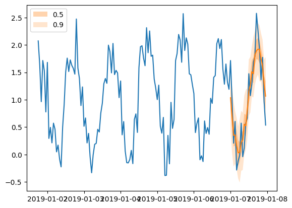
[76]:
plt.plot(tss[0][-150:].to_timestamp())
forecasts[0].plot(show_label=True)
plt.legend()
[76]:
<matplotlib.legend.Legend at 0x7f249808ac40>
添加特征和缩放#
在之前的网络中,我们只使用了 target,没有利用数据集的任何特征。在这里,我们通过包含数据集的 feat_dynamic_real 字段来扩展概率网络,这可以增强模型的预测能力。我们通过将 target 和特征连接成一个新的增强向量来形成新的网络输入,从而实现这一点。
数据集中所有可用的特征都可以作为我们模型的输入。然而,为了本示例的目的,我们将限制自己仅使用一个特征。
实践者经常需要处理的一个重要问题是数据集中时间序列值的数量级不同。对于在大致相同值范围内训练和预测值的模型来说,这非常有帮助。为了解决这个问题,我们在模型中添加了一个 Scaler,它计算每个时间序列的比例。然后我们可以相应地缩放时间序列的值或任何相关特征,并将这些作为网络的输入。
[77]:
from gluonts.mx import MeanScaler, NOPScaler
[78]:
class MyProbNetwork(gluon.HybridBlock):
    def __init__(
        self,
        prediction_length,
        context_length,
        distr_output,
        num_cells,
        num_sample_paths=100,
        scaling=True,
        **kwargs
    ) -> None:
        super().__init__(**kwargs)
        self.prediction_length = prediction_length
        self.context_length = context_length
        self.distr_output = distr_output
        self.num_cells = num_cells
        self.num_sample_paths = num_sample_paths
        self.proj_distr_args = distr_output.get_args_proj()
        self.scaling = scaling

        with self.name_scope():
            # Set up a 2 layer neural network that its ouput will be projected to the distribution parameters
            self.nn = mx.gluon.nn.HybridSequential()
            self.nn.add(mx.gluon.nn.Dense(units=self.num_cells, activation="relu"))
            self.nn.add(
                mx.gluon.nn.Dense(
                    units=self.prediction_length * self.num_cells, activation="relu"
                )
            )

            if scaling:
                self.scaler = MeanScaler(keepdims=True)
            else:
                self.scaler = NOPScaler(keepdims=True)

    def compute_scale(self, past_target, past_observed_values):
        # scale shape is (batch_size, 1)
        _, scale = self.scaler(
            past_target.slice_axis(axis=1, begin=-self.context_length, end=None),
            past_observed_values.slice_axis(
                axis=1, begin=-self.context_length, end=None
            ),
        )

        return scale


class MyProbTrainNetwork(MyProbNetwork):
    def hybrid_forward(
        self,
        F,
        past_target,
        future_target,
        past_observed_values,
        past_feat_dynamic_real,
    ):
        # compute scale
        scale = self.compute_scale(past_target, past_observed_values)

        # scale target and time features
        past_target_scale = F.broadcast_div(past_target, scale)
        past_feat_dynamic_real_scale = F.broadcast_div(
            past_feat_dynamic_real.squeeze(axis=-1), scale
        )

        # concatenate target and time features to use them as input to the network
        net_input = F.concat(past_target_scale, past_feat_dynamic_real_scale, dim=-1)

        # compute network output
        net_output = self.nn(net_input)

        # (batch, prediction_length * nn_features)  ->  (batch, prediction_length, nn_features)
        net_output = net_output.reshape(0, self.prediction_length, -1)

        # project network output to distribution parameters domain
        distr_args = self.proj_distr_args(net_output)

        # compute distribution
        distr = self.distr_output.distribution(distr_args, scale=scale)

        # negative log-likelihood
        loss = distr.loss(future_target)
        return loss


class MyProbPredNetwork(MyProbTrainNetwork):
    # The prediction network only receives past_target and returns predictions
    def hybrid_forward(
        self, F, past_target, past_observed_values, past_feat_dynamic_real
    ):
        # repeat fields: from (batch_size, past_target_length) to
        # (batch_size * num_sample_paths, past_target_length)
        repeated_past_target = past_target.repeat(repeats=self.num_sample_paths, axis=0)
        repeated_past_observed_values = past_observed_values.repeat(
            repeats=self.num_sample_paths, axis=0
        )
        repeated_past_feat_dynamic_real = past_feat_dynamic_real.repeat(
            repeats=self.num_sample_paths, axis=0
        )

        # compute scale
        scale = self.compute_scale(repeated_past_target, repeated_past_observed_values)

        # scale repeated target and time features
        repeated_past_target_scale = F.broadcast_div(repeated_past_target, scale)
        repeated_past_feat_dynamic_real_scale = F.broadcast_div(
            repeated_past_feat_dynamic_real.squeeze(axis=-1), scale
        )

        # concatenate target and time features to use them as input to the network
        net_input = F.concat(
            repeated_past_target_scale, repeated_past_feat_dynamic_real_scale, dim=-1
        )

        # compute network oputput
        net_output = self.nn(net_input)

        # (batch * num_sample_paths, prediction_length * nn_features)  ->  (batch * num_sample_paths, prediction_length, nn_features)
        net_output = net_output.reshape(0, self.prediction_length, -1)

        # project network output to distribution parameters domain
        distr_args = self.proj_distr_args(net_output)

        # compute distribution
        distr = self.distr_output.distribution(distr_args, scale=scale)

        # get (batch_size * num_sample_paths, prediction_length) samples
        samples = distr.sample()

        # reshape from (batch_size * num_sample_paths, prediction_length) to
        # (batch_size, num_sample_paths, prediction_length)
        return samples.reshape(
            shape=(-1, self.num_sample_paths, self.prediction_length)
        )
[79]:
class MyProbEstimator(GluonEstimator):
    @validated()
    def __init__(
        self,
        prediction_length: int,
        context_length: int,
        distr_output: DistributionOutput,
        num_cells: int,
        num_sample_paths: int = 100,
        scaling: bool = True,
        batch_size: int = 32,
        trainer: Trainer = Trainer(),
    ) -> None:
        super().__init__(trainer=trainer, batch_size=batch_size)
        self.prediction_length = prediction_length
        self.context_length = context_length
        self.distr_output = distr_output
        self.num_cells = num_cells
        self.num_sample_paths = num_sample_paths
        self.scaling = scaling

    def create_transformation(self):
        # Feature transformation that the model uses for input.
        return AddObservedValuesIndicator(
            target_field=FieldName.TARGET,
            output_field=FieldName.OBSERVED_VALUES,
        )

    def create_training_data_loader(self, dataset, **kwargs):
        instance_splitter = InstanceSplitter(
            target_field=FieldName.TARGET,
            is_pad_field=FieldName.IS_PAD,
            start_field=FieldName.START,
            forecast_start_field=FieldName.FORECAST_START,
            instance_sampler=ExpectedNumInstanceSampler(
                num_instances=1, min_future=self.prediction_length
            ),
            past_length=self.context_length,
            future_length=self.prediction_length,
            time_series_fields=[
                FieldName.FEAT_DYNAMIC_REAL,
                FieldName.OBSERVED_VALUES,
            ],
        )
        input_names = get_hybrid_forward_input_names(MyProbTrainNetwork)
        return TrainDataLoader(
            dataset=dataset,
            transform=instance_splitter + SelectFields(input_names),
            batch_size=self.batch_size,
            stack_fn=partial(batchify, ctx=self.trainer.ctx, dtype=self.dtype),
            **kwargs,
        )

    def create_training_network(self) -> MyProbTrainNetwork:
        return MyProbTrainNetwork(
            prediction_length=self.prediction_length,
            context_length=self.context_length,
            distr_output=self.distr_output,
            num_cells=self.num_cells,
            num_sample_paths=self.num_sample_paths,
            scaling=self.scaling,
        )

    def create_predictor(
        self, transformation: Transformation, trained_network: HybridBlock
    ) -> Predictor:
        prediction_splitter = InstanceSplitter(
            target_field=FieldName.TARGET,
            is_pad_field=FieldName.IS_PAD,
            start_field=FieldName.START,
            forecast_start_field=FieldName.FORECAST_START,
            instance_sampler=TestSplitSampler(),
            past_length=self.context_length,
            future_length=self.prediction_length,
            time_series_fields=[
                FieldName.FEAT_DYNAMIC_REAL,
                FieldName.OBSERVED_VALUES,
            ],
        )

        prediction_network = MyProbPredNetwork(
            prediction_length=self.prediction_length,
            context_length=self.context_length,
            distr_output=self.distr_output,
            num_cells=self.num_cells,
            num_sample_paths=self.num_sample_paths,
            scaling=self.scaling,
        )

        copy_parameters(trained_network, prediction_network)

        return RepresentableBlockPredictor(
            input_transform=transformation + prediction_splitter,
            prediction_net=prediction_network,
            batch_size=self.batch_size,
            prediction_length=self.prediction_length,
            ctx=self.trainer.ctx,
        )
[80]:
estimator = MyProbEstimator(
    prediction_length=custom_ds_metadata["prediction_length"],
    context_length=2 * custom_ds_metadata["prediction_length"],
    distr_output=GaussianOutput(),
    num_cells=40,
    trainer=Trainer(
        ctx="cpu",
        epochs=5,
        learning_rate=1e-3,
        hybridize=False,
        num_batches_per_epoch=100,
    ),
)
[81]:
predictor = estimator.train(train_ds)
100%|██████████| 100/100 [00:00<00:00, 119.95it/s, epoch=1/5, avg_epoch_loss=0.967]
100%|██████████| 100/100 [00:00<00:00, 123.75it/s, epoch=2/5, avg_epoch_loss=0.536]
100%|██████████| 100/100 [00:00<00:00, 135.19it/s, epoch=3/5, avg_epoch_loss=0.483]
100%|██████████| 100/100 [00:00<00:00, 126.54it/s, epoch=4/5, avg_epoch_loss=0.455]
100%|██████████| 100/100 [00:00<00:00, 122.88it/s, epoch=5/5, avg_epoch_loss=0.431]
[82]:
forecast_it, ts_it = make_evaluation_predictions(
    dataset=test_ds,  # test dataset
    predictor=predictor,  # predictor
    num_samples=100,  # number of sample paths we want for evaluation
)
[83]:
forecasts = list(forecast_it)
tss = list(ts_it)
[84]:
plt.plot(tss[0][-150:].to_timestamp())
forecasts[0].plot(show_label=True)
plt.legend()
[84]:
<matplotlib.legend.Legend at 0x7f24cf974ac0>
从前馈网络到 RNN#
在所有之前的示例中,我们都使用了前馈神经网络作为预测模型的基础。其主要思想是使用时间序列的一个窗口(长度为 context_length)作为网络输入,并训练网络预测随后的窗口(长度为 prediction_length)。
在本节中,我们将用循环神经网络(RNN)替换前馈网络。由于 RNN 的性质不同,网络的结构也会有所不同。让我们看看主要变化有哪些。
训练#
RNN 的主要思想与我们之前构建的前馈网络相同:在每个时间步展开 RNN 时,我们使用时间序列的过去值作为输入并预测下一个值。我们可以通过使用多个过去值(例如基于季节性模式的特定滞后)或可用特征来增强输入。然而,在本示例中,我们将保持简单,仅使用时间序列的最后一个值。网络在每个时间步的输出是下一个时间步值的分布,其中 RNN 的状态用作分布参数投影的特征向量。
由于 RNN 的顺序性质,在时间序列的切割窗口中区分 past_ 和 future_ 实际上不是必需的。因此,我们可以将 past_target 和 future_target 连接起来,并将其视为我们希望预测的具体 target 窗口。这意味着 RNN 的输入将是(顺序地)窗口 target[-(context_length + prediction_length + 1):-1](比我们想预测的窗口提前一个时间步)。因此,我们需要在切割的每个窗口中具有 context_length + prediction_length + 1 个可用值。我们可以在 InstanceSplitter 中定义这一点。
总的来说,训练期间的步骤如下:
我们按顺序将 target 值
target[-(context_length + prediction_length + 1):-1]通过 RNN我们将 RNN 在每个时间步的状态用作特征向量,并将其投影到分布参数域
每个时间步的输出是下一个时间步值的分布,总体而言,这就是窗口
target[-(context_length + prediction_length):]的预测分布。
上述步骤在 unroll_encoder 方法中实现。
推理#
在推理过程中,我们只知道 past_target 的值,因此无法完全遵循训练中的相同步骤。但是主要思想非常相似:
我们按顺序将过去的 target 值
past_target[-(context_length + 1):]通过 RNN,这有效地更新了 RNN 的状态在最后一个时间步,RNN 的输出实际上是时间序列下一个值(我们不知道)的分布。因此,我们从此分布中采样(
num_sample_paths次),并将样本用作 RNN 下一个时间步的输入。我们重复上一步
prediction_length次
第一步在 unroll_encoder 中实现,最后几步在 sample_decoder 方法中实现。
[85]:
class MyProbRNN(gluon.HybridBlock):
    def __init__(
        self,
        prediction_length,
        context_length,
        distr_output,
        num_cells,
        num_layers,
        num_sample_paths=100,
        scaling=True,
        **kwargs
    ) -> None:
        super().__init__(**kwargs)
        self.prediction_length = prediction_length
        self.context_length = context_length
        self.distr_output = distr_output
        self.num_cells = num_cells
        self.num_layers = num_layers
        self.num_sample_paths = num_sample_paths
        self.proj_distr_args = distr_output.get_args_proj()
        self.scaling = scaling

        with self.name_scope():
            self.rnn = mx.gluon.rnn.HybridSequentialRNNCell()
            for k in range(self.num_layers):
                cell = mx.gluon.rnn.LSTMCell(hidden_size=self.num_cells)
                cell = mx.gluon.rnn.ResidualCell(cell) if k > 0 else cell
                self.rnn.add(cell)

            if scaling:
                self.scaler = MeanScaler(keepdims=True)
            else:
                self.scaler = NOPScaler(keepdims=True)

    def compute_scale(self, past_target, past_observed_values):
        # scale is computed on the context length last units of the past target
        # scale shape is (batch_size, 1, *target_shape)
        _, scale = self.scaler(
            past_target.slice_axis(axis=1, begin=-self.context_length, end=None),
            past_observed_values.slice_axis(
                axis=1, begin=-self.context_length, end=None
            ),
        )

        return scale

    def unroll_encoder(
        self,
        F,
        past_target,
        past_observed_values,
        future_target=None,
        future_observed_values=None,
    ):
        # overall target field
        # input target from -(context_length + prediction_length + 1) to -1
        if future_target is not None:  # during training
            target_in = F.concat(past_target, future_target, dim=-1).slice_axis(
                axis=1,
                begin=-(self.context_length + self.prediction_length + 1),
                end=-1,
            )

            # overall observed_values field
            # input observed_values corresponding to target_in
            observed_values_in = F.concat(
                past_observed_values, future_observed_values, dim=-1
            ).slice_axis(
                axis=1,
                begin=-(self.context_length + self.prediction_length + 1),
                end=-1,
            )

            rnn_length = self.context_length + self.prediction_length
        else:  # during inference
            target_in = past_target.slice_axis(
                axis=1, begin=-(self.context_length + 1), end=-1
            )

            # overall observed_values field
            # input observed_values corresponding to target_in
            observed_values_in = past_observed_values.slice_axis(
                axis=1, begin=-(self.context_length + 1), end=-1
            )

            rnn_length = self.context_length

        # compute scale
        scale = self.compute_scale(target_in, observed_values_in)

        # scale target_in
        target_in_scale = F.broadcast_div(target_in, scale)

        # compute network output
        net_output, states = self.rnn.unroll(
            inputs=target_in_scale,
            length=rnn_length,
            layout="NTC",
            merge_outputs=True,
        )

        return net_output, states, scale


class MyProbTrainRNN(MyProbRNN):
    def hybrid_forward(
        self,
        F,
        past_target,
        future_target,
        past_observed_values,
        future_observed_values,
    ):
        net_output, _, scale = self.unroll_encoder(
            F, past_target, past_observed_values, future_target, future_observed_values
        )

        # output target from -(context_length + prediction_length) to end
        target_out = F.concat(past_target, future_target, dim=-1).slice_axis(
            axis=1, begin=-(self.context_length + self.prediction_length), end=None
        )

        # project network output to distribution parameters domain
        distr_args = self.proj_distr_args(net_output)

        # compute distribution
        distr = self.distr_output.distribution(distr_args, scale=scale)

        # negative log-likelihood
        loss = distr.loss(target_out)
        return loss


class MyProbPredRNN(MyProbTrainRNN):
    def sample_decoder(self, F, past_target, states, scale):
        # repeat fields: from (batch_size, past_target_length) to
        # (batch_size * num_sample_paths, past_target_length)
        repeated_states = [
            s.repeat(repeats=self.num_sample_paths, axis=0) for s in states
        ]
        repeated_scale = scale.repeat(repeats=self.num_sample_paths, axis=0)

        # first decoder input is the last value of the past_target, i.e.,
        # the previous value of the first time step we want to forecast
        decoder_input = past_target.slice_axis(axis=1, begin=-1, end=None).repeat(
            repeats=self.num_sample_paths, axis=0
        )

        # list with samples at each time step
        future_samples = []

        # for each future time step we draw new samples for this time step and update the state
        # the drawn samples are the inputs to the rnn at the next time step
        for k in range(self.prediction_length):
            rnn_outputs, repeated_states = self.rnn.unroll(
                inputs=decoder_input,
                length=1,
                begin_state=repeated_states,
                layout="NTC",
                merge_outputs=True,
            )

            # project network output to distribution parameters domain
            distr_args = self.proj_distr_args(rnn_outputs)

            # compute distribution
            distr = self.distr_output.distribution(distr_args, scale=repeated_scale)

            # draw samples (batch_size * num_samples, 1)
            new_samples = distr.sample()

            # append the samples of the current time step
            future_samples.append(new_samples)

            # update decoder input for the next time step
            decoder_input = new_samples

        samples = F.concat(*future_samples, dim=1)

        # (batch_size, num_samples, prediction_length)
        return samples.reshape(
            shape=(-1, self.num_sample_paths, self.prediction_length)
        )

    def hybrid_forward(self, F, past_target, past_observed_values):
        # unroll encoder over context_length
        net_output, states, scale = self.unroll_encoder(
            F, past_target, past_observed_values
        )

        samples = self.sample_decoder(F, past_target, states, scale)

        return samples
[86]:
class MyProbRNNEstimator(GluonEstimator):
    @validated()
    def __init__(
        self,
        prediction_length: int,
        context_length: int,
        distr_output: DistributionOutput,
        num_cells: int,
        num_layers: int,
        num_sample_paths: int = 100,
        scaling: bool = True,
        batch_size: int = 32,
        trainer: Trainer = Trainer(),
    ) -> None:
        super().__init__(trainer=trainer, batch_size=batch_size)
        self.prediction_length = prediction_length
        self.context_length = context_length
        self.distr_output = distr_output
        self.num_cells = num_cells
        self.num_layers = num_layers
        self.num_sample_paths = num_sample_paths
        self.scaling = scaling

    def create_transformation(self):
        # Feature transformation that the model uses for input.
        return AddObservedValuesIndicator(
            target_field=FieldName.TARGET,
            output_field=FieldName.OBSERVED_VALUES,
        )

    def create_training_data_loader(self, dataset, **kwargs):
        instance_splitter = InstanceSplitter(
            target_field=FieldName.TARGET,
            is_pad_field=FieldName.IS_PAD,
            start_field=FieldName.START,
            forecast_start_field=FieldName.FORECAST_START,
            instance_sampler=ExpectedNumInstanceSampler(
                num_instances=1,
                min_future=self.prediction_length,
            ),
            past_length=self.context_length + 1,
            future_length=self.prediction_length,
            time_series_fields=[
                FieldName.FEAT_DYNAMIC_REAL,
                FieldName.OBSERVED_VALUES,
            ],
        )
        input_names = get_hybrid_forward_input_names(MyProbTrainRNN)
        return TrainDataLoader(
            dataset=dataset,
            transform=instance_splitter + SelectFields(input_names),
            batch_size=self.batch_size,
            stack_fn=partial(batchify, ctx=self.trainer.ctx, dtype=self.dtype),
            **kwargs,
        )

    def create_training_network(self) -> MyProbTrainRNN:
        return MyProbTrainRNN(
            prediction_length=self.prediction_length,
            context_length=self.context_length,
            distr_output=self.distr_output,
            num_cells=self.num_cells,
            num_layers=self.num_layers,
            num_sample_paths=self.num_sample_paths,
            scaling=self.scaling,
        )

    def create_predictor(
        self, transformation: Transformation, trained_network: HybridBlock
    ) -> Predictor:
        prediction_splitter = InstanceSplitter(
            target_field=FieldName.TARGET,
            is_pad_field=FieldName.IS_PAD,
            start_field=FieldName.START,
            forecast_start_field=FieldName.FORECAST_START,
            instance_sampler=TestSplitSampler(),
            past_length=self.context_length + 1,
            future_length=self.prediction_length,
            time_series_fields=[
                FieldName.FEAT_DYNAMIC_REAL,
                FieldName.OBSERVED_VALUES,
            ],
        )
        prediction_network = MyProbPredRNN(
            prediction_length=self.prediction_length,
            context_length=self.context_length,
            distr_output=self.distr_output,
            num_cells=self.num_cells,
            num_layers=self.num_layers,
            num_sample_paths=self.num_sample_paths,
            scaling=self.scaling,
        )

        copy_parameters(trained_network, prediction_network)

        return RepresentableBlockPredictor(
            input_transform=transformation + prediction_splitter,
            prediction_net=prediction_network,
            batch_size=self.batch_size,
            prediction_length=self.prediction_length,
            ctx=self.trainer.ctx,
        )
[87]:
estimator = MyProbRNNEstimator(
    prediction_length=24,
    context_length=48,
    num_cells=40,
    num_layers=2,
    distr_output=GaussianOutput(),
    trainer=Trainer(
        ctx="cpu",
        epochs=5,
        learning_rate=1e-3,
        hybridize=False,
        num_batches_per_epoch=100,
    ),
)
[88]:
predictor = estimator.train(train_ds)
100%|██████████| 100/100 [00:16<00:00,  6.03it/s, epoch=1/5, avg_epoch_loss=0.752]
100%|██████████| 100/100 [00:16<00:00,  6.03it/s, epoch=2/5, avg_epoch_loss=0.394]
100%|██████████| 100/100 [00:16<00:00,  5.88it/s, epoch=3/5, avg_epoch_loss=0.342]
100%|██████████| 100/100 [00:16<00:00,  6.06it/s, epoch=4/5, avg_epoch_loss=0.294]
100%|██████████| 100/100 [00:16<00:00,  5.96it/s, epoch=5/5, avg_epoch_loss=0.268]
[89]:
forecast_it, ts_it = make_evaluation_predictions(
    dataset=test_ds,  # test dataset
    predictor=predictor,  # predictor
    num_samples=100,  # number of sample paths we want for evaluation
)
[90]:
forecasts = list(forecast_it)
tss = list(ts_it)
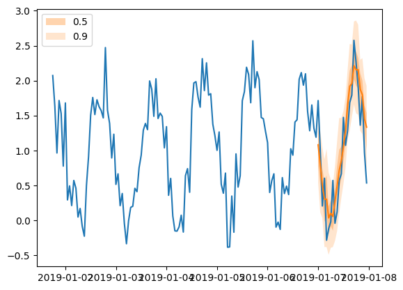
[91]:
plt.plot(tss[0][-150:].to_timestamp())
forecasts[0].plot(show_label=True)
plt.legend()
[91]:
<matplotlib.legend.Legend at 0x7f2498159640>